library(hmisindia)
library(dplyr)
library(ggplot2)
library(tidyr)
library(DT)

data_available <- tryCatch(
  {
    pq <- hmisindia::get_parquet_path()
    nzchar(pq) && file.exists(pq)
  },
  error = function(e) FALSE
)
knitr::opts_chunk$set(eval = data_available)
The hmisindia package provides access to India’s Health
Management Information System (HMIS) data: 840+ health indicators across
36 states/UTs from April 2008 to December 2024, with district-level data
for 700+ districts.
Browsing indicators
Find what’s available with list_indicators() and
search_indicators():
# All state-level indicators
list_indicators()
#> # A tibble: 840 × 4
#>    canonical_name                               n_yearmon first_month last_month
#>    <chr>                                            <dbl> <chr>       <chr>
#>  1 Above 10 years to below 19 years                    24 Apr 2023    Mar 2025
#>  2 Above 5 years to below 10 years                     24 Apr 2023    Mar 2025
#>  3 Adult above >19 years                               24 Apr 2023    Mar 2025
#>  4 Albendazole 400 mg tablet                           96 Apr 2017    Mar 2025
#>  5 Amoxycillin (Paediatrics Antibiotics)               24 Apr 2023    Mar 2025
#>  6 Antepartum (Macerated) Still Birth                  24 Apr 2023    Mar 2025
#>  7 Average kilometres travelled by ALS during …        24 Apr 2023    Mar 2025
#>  8 Average kilometres travelled by BLS during …        24 Apr 2023    Mar 2025
#>  9 Average number of trips per day by ALS duri…        24 Apr 2023    Mar 2025
#> 10 Average number of trips per day by BLS duri…        24 Apr 2023    Mar 2025
#> # ℹ 830 more rows

# Search by keyword
search_indicators("malaria")
#> # A tibble: 14 × 4
#>    canonical_name                               n_yearmon first_month last_month
#>    <chr>                                            <dbl> <chr>       <chr>
#>  1 Childhood Diseases - Malaria                        96 Apr 2017    Mar 2025
#>  2 Inpatient - Malaria                                 96 Apr 2017    Mar 2025
#>  3 Malaria (Microscopy Tests) - Mixed test pos…        24 Apr 2023    Mar 2025
#>  4 Malaria (Microscopy Tests) - Plasmodium Fal…        96 Apr 2017    Mar 2025
#>  5 Malaria (Microscopy Tests) - Plasmodium Viv…        96 Apr 2017    Mar 2025
#>  6 Malaria (RDT) - Plamodium Falciparum test p…        96 Apr 2017    Mar 2025
#>  7 Number of blood smears examined for Malaria        204 Apr 2008    Mar 2025
#>  8 Number of cases of Adolescent or Adult deat…       108 Apr 2008    Mar 2017
#>  9 Number of cases of Malaria reported in chil…       108 Apr 2008    Mar 2017
#> 10 Number of Deaths due to Malaria - Plasmodiu…        96 Apr 2017    Mar 2025
#> 11 Number of Deaths due to Malaria - Plasmodiu…        96 Apr 2017    Mar 2025
#> 12 Out of blood smears examined for malaria, n…       108 Apr 2008    Mar 2017
#> 13 Out of blood smears examined for malaria, n…       108 Apr 2008    Mar 2017
#> 14 RDT conducted for Malaria                           96 Apr 2017    Mar 2025

# District-level indicators
search_indicators("live birth", geography = "district")
#> # A tibble: 4 × 4
#>   canonical_name                                n_yearmon first_month last_month
#>   <chr>                                             <int> <chr>       <chr>
#> 1 Number of female live births                        204 Apr 2008    Mar 2025
#> 2 Number of live births among Syphilis Seropos…        24 Apr 2023    Mar 2025
#> 3 Number of male live births                          204 Apr 2008    Mar 2025
#> 4 Total number of male and female live births …       108 Apr 2008    Mar 2017
Querying data
get_hmis() queries indicator data by substring match
(default), regex, or fuzzy match:
# All data for an indicator
births <- get_hmis("Number of female live births",
  category = "Total",
  sector = "Total"
)
datatable(births, options = list(pageLength = 10, scrollX = TRUE))
Filter by state, time period, and more:
Time series plots
plot_time_series() creates line plots colored by state
(or district, indicator, etc.):
plot_time_series(births_subset, y_label = "Number of live births (female)")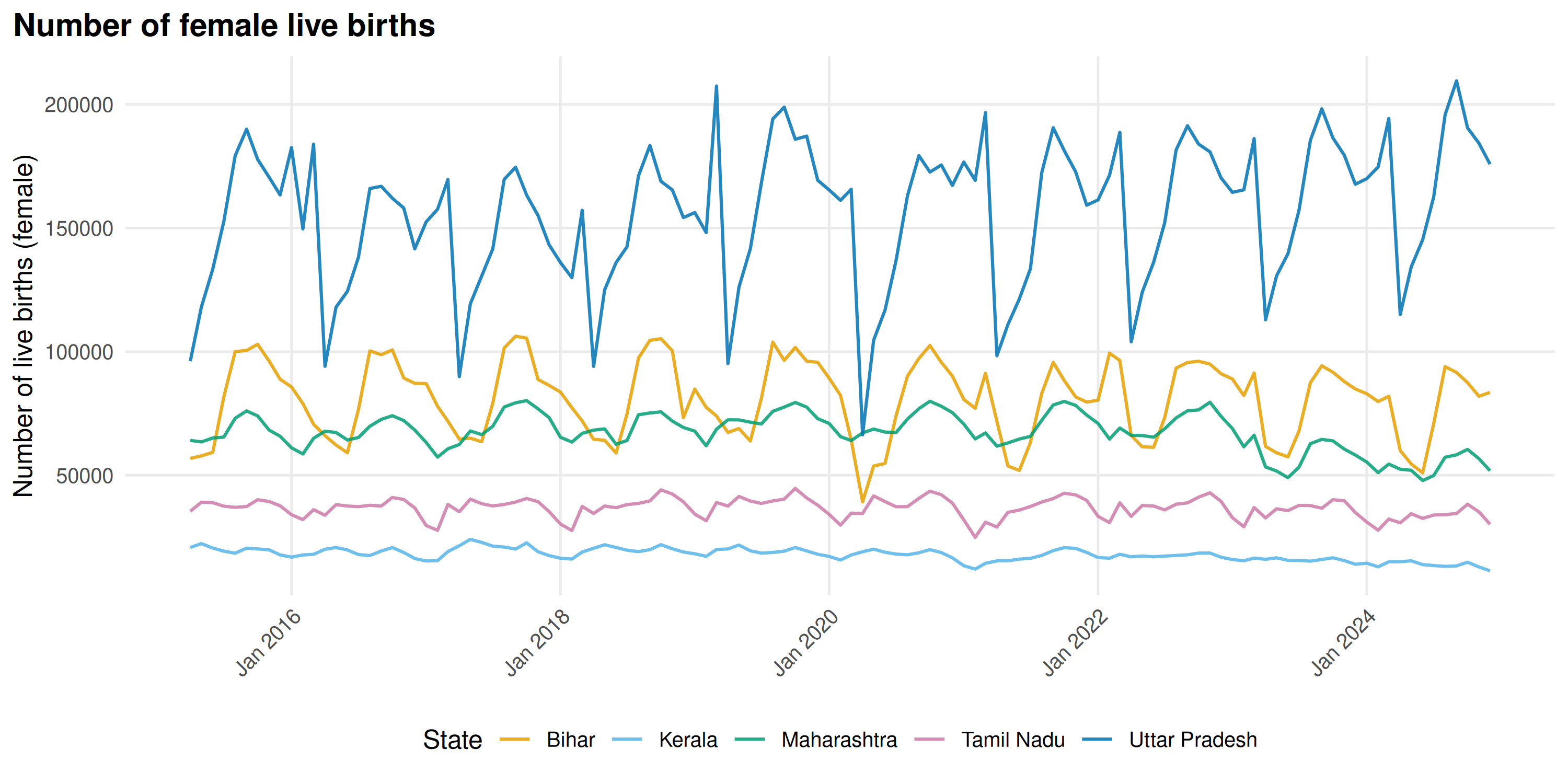
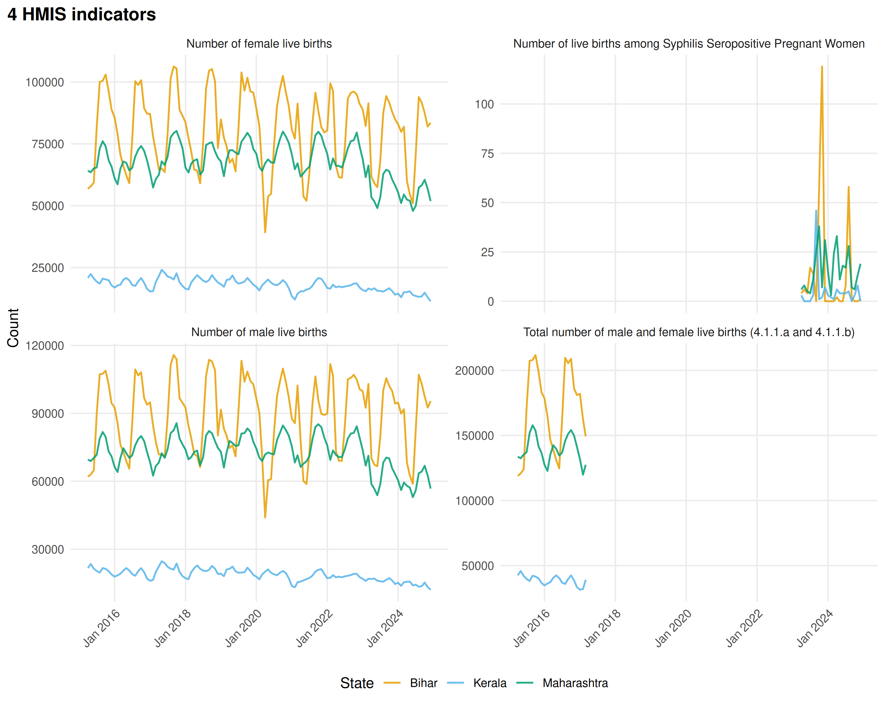
Compare multiple indicators by faceting:
birth_indicators <- get_hmis("live births",
  state = c("Bihar", "Kerala", "Maharashtra"),
  category = "Total",
  sector = "Total",
  from = "Apr 2015",
  to = "Dec 2024"
)

plot_time_series(birth_indicators,
  facet = "canonical_name",
  y_label = "Count"
)
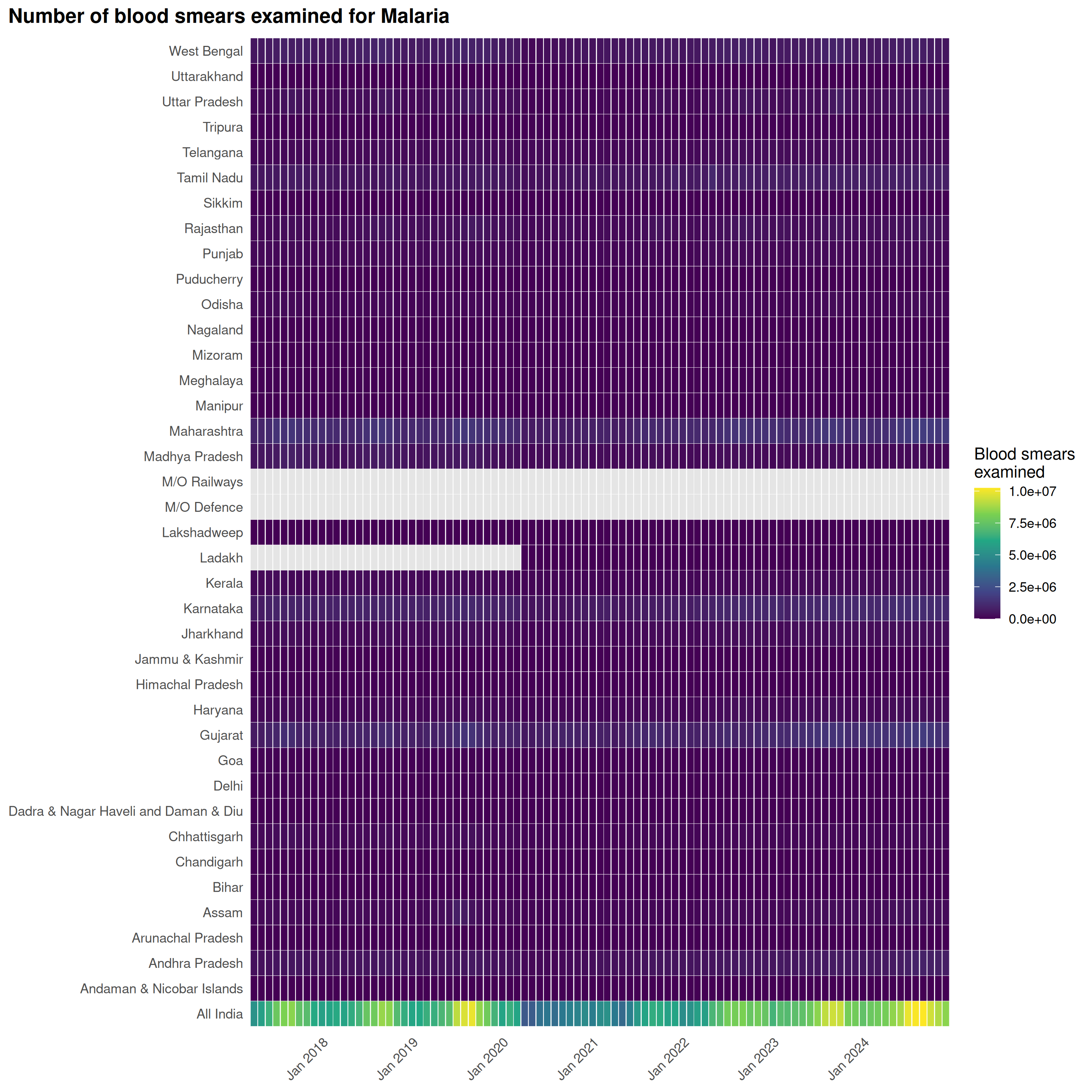
Heatmaps
plot_heatmap() shows values across states and time:
malaria <- get_hmis("Number of blood smears examined for Malaria",
  category = "Total",
  sector = "Total",
  from = "Apr 2017",
  to = "Dec 2024"
)
plot_heatmap(malaria,
  legend_title = "Blood smears\nexamined",
  palette = "viridis"
)
Scatter plots
plot_scatter() compares two variables. Here we compare
male vs female live births:
male_births <- get_hmis("Number of male live births",
  category = "Total",
  sector = "Total",
  from = "Apr 2015",
  to = "Dec 2024"
)
female_births <- get_hmis("Number of female live births",
  category = "Total",
  sector = "Total",
  from = "Apr 2015",
  to = "Dec 2024"
)

# Merge the two indicators into wide format
scatter_data <- inner_join(
  male_births |> select(state, monyear, male = value),
  female_births |> select(state, monyear, female = value),
  by = c("state", "monyear")
)
plot_scatter(scatter_data,
  x = "male",
  y = "female",
  x_label = "Male live births",
  y_label = "Female live births",
  title = "Male vs female live births across states"
)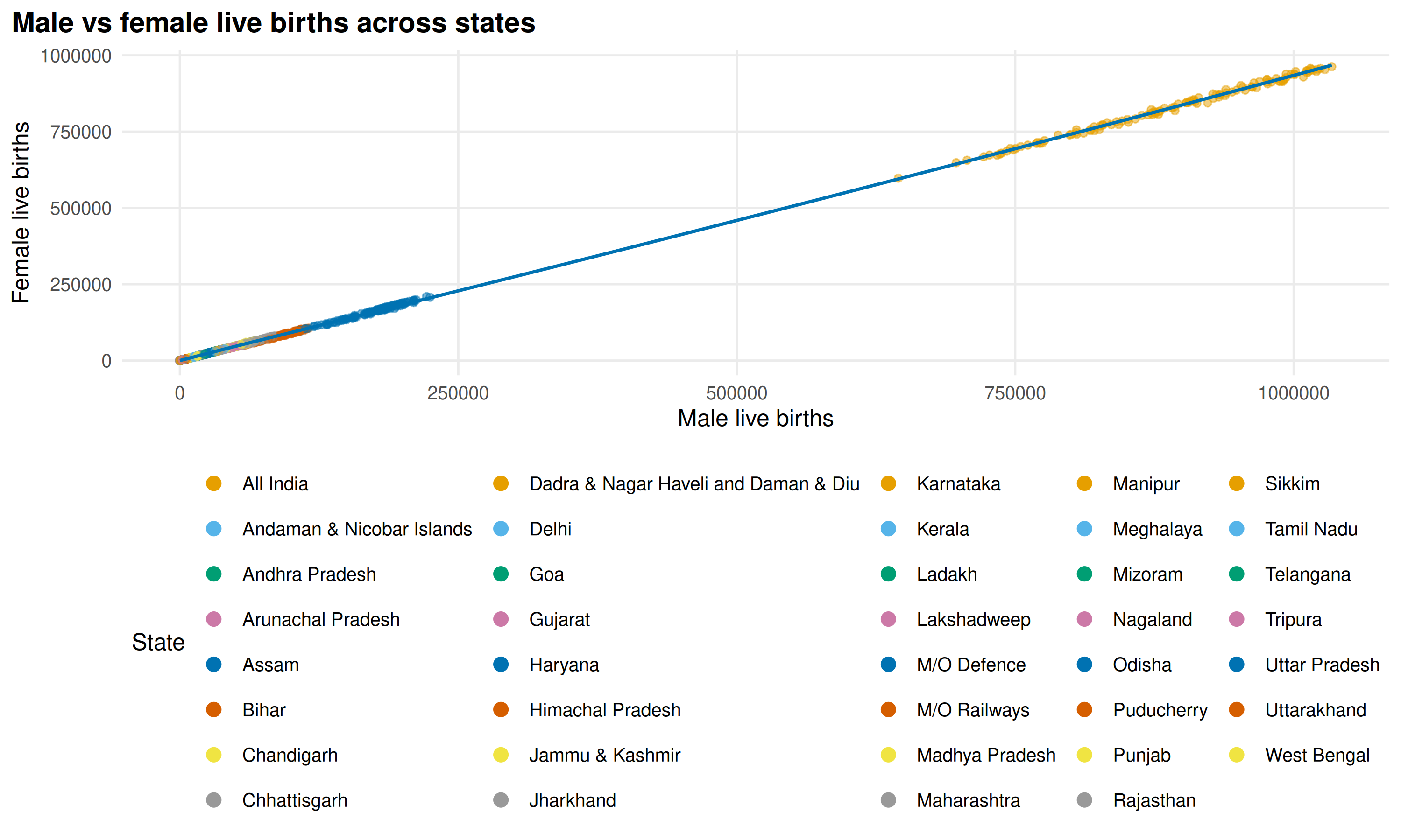
Sex ratios at birth are consistent across states and time.
Periodicity detection
detect_periodicity() tests for seasonal patterns using
spectral analysis and autocorrelation:
kerala_births <- get_hmis("Number of female live births",
  state = "Kerala",
  category = "Total",
  sector = "Total"
)

prd <- detect_periodicity(kerala_births)
print(prd)
#> Periodicity analysis (n = 204 observations)
#>   Detrended: TRUE
#>   Dominant period: 6.2 observations
#>   Spectral power concentration: 6.4 %
#>   ACF at dominant lag: 0.305 (threshold: 0.137 )
#>
#> Top frequencies:
#>  period    power
#>    6.17 19215478
#>    6.00 19009942
#>    5.84 18639115
#>    6.35 18599844
#>    5.68 18036973
plot(prd)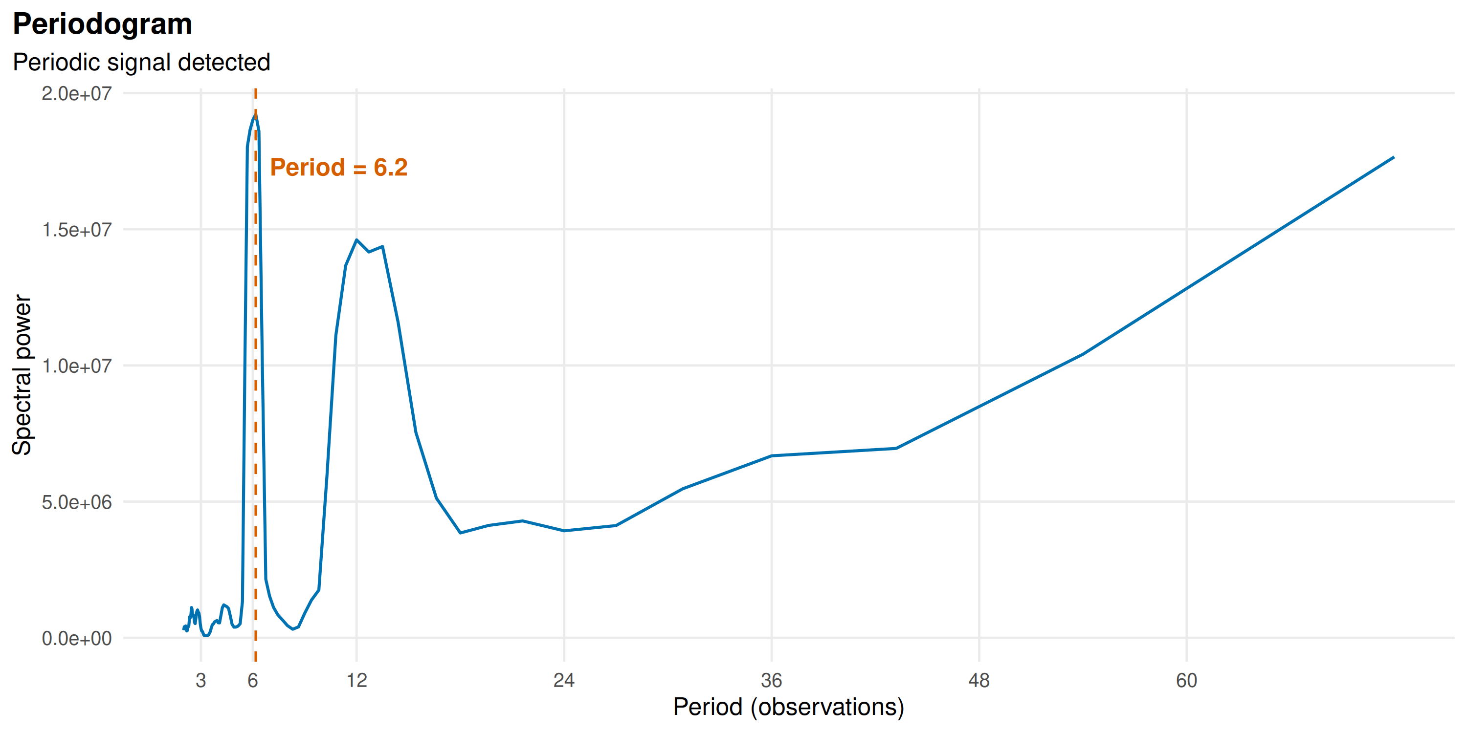
A spectral peak at 12 months indicates an annual cycle.
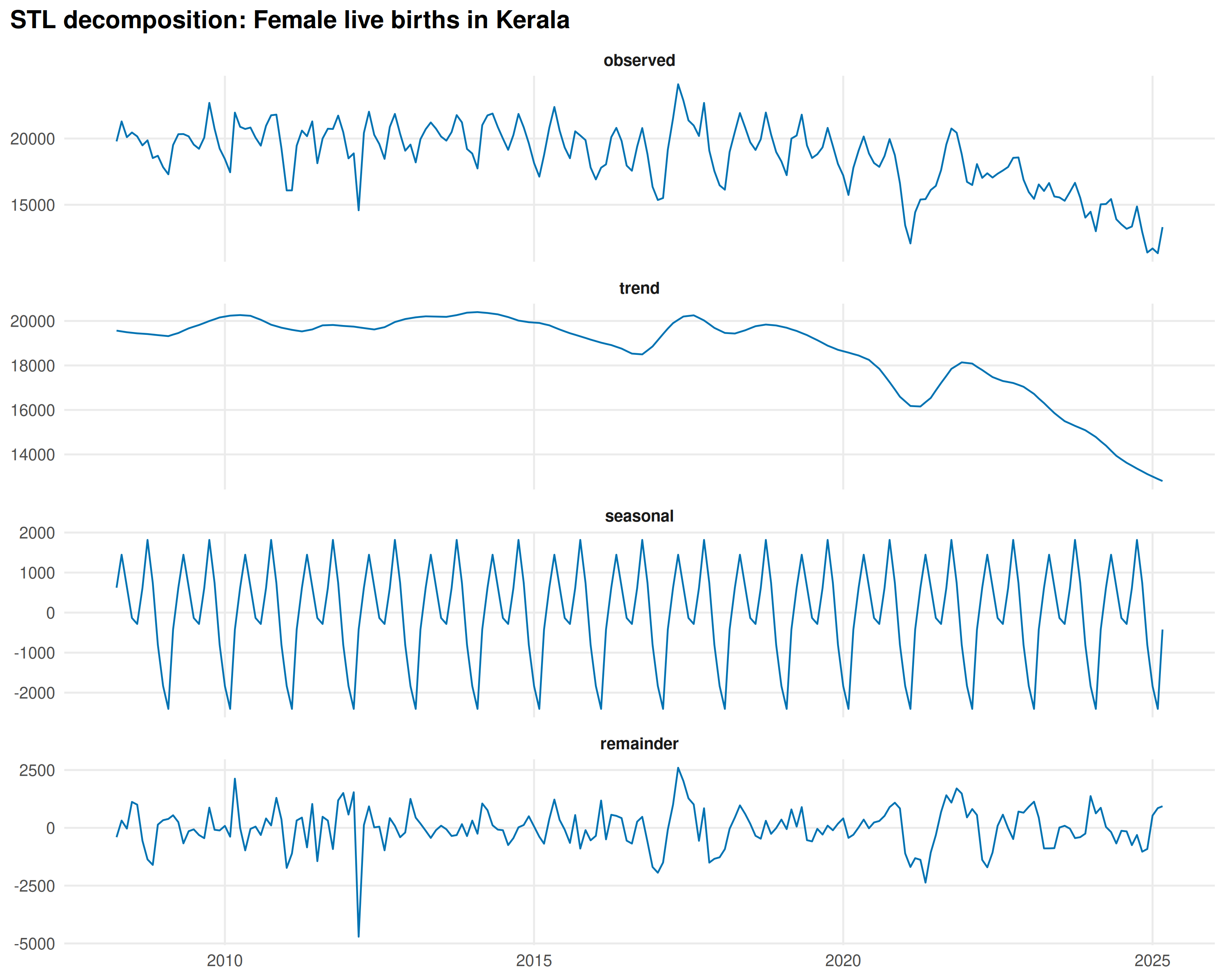
Decomposing seasonal components
decompose_series() separates trend, seasonal, and
residual components using STL decomposition:
decomp <- decompose_series(kerala_births)

decomp_long <- decomp |>
  pivot_longer(
    cols = c(observed, trend, seasonal, remainder),
    names_to = "component",
    values_to = "val"
  ) |>
  mutate(component = factor(component,
    levels = c("observed", "trend", "seasonal", "remainder")
  ))

ggplot(decomp_long, aes(date, val)) +
  geom_line(color = "#0072B2", linewidth = 0.5) +
  facet_wrap(~component, ncol = 1, scales = "free_y") +
  labs(
    x = NULL, y = NULL,
    title = "STL decomposition: Female live births in Kerala"
  ) +
  theme_minimal(base_size = 12) +
  theme(
    strip.text = element_text(face = "bold"),
    panel.grid.minor = element_blank(),
    plot.title = element_text(face = "bold"),
    plot.title.position = "plot"
  )
District-level data
Query district data by setting
geography = "district":
# List districts in a state
list_districts(state = "Bihar")
#> # A tibble: 38 × 2
#>    state district
#>    <chr> <chr>
#>  1 Bihar Araria
#>  2 Bihar Arwal
#>  3 Bihar Aurangabad
#>  4 Bihar Banka
#>  5 Bihar Begusarai
#>  6 Bihar Bhagalpur
#>  7 Bihar Bhojpur
#>  8 Bihar Buxar
#>  9 Bihar Darbhanga
#> 10 Bihar Gaya
#> # ℹ 28 more rows
# District-level malaria data
bihar_malaria <- get_hmis("Number of blood smears examined for Malaria",
  geography = "district",
  state = "Bihar",
  category = "Total",
  sector = "Total",
  from = "Apr 2020",
  to = "Dec 2024"
)
# Show top 8 districts by volume
top_districts <- bihar_malaria |>
  group_by(district) |>
  summarise(total = sum(value, na.rm = TRUE)) |>
  slice_max(total, n = 8) |>
  pull(district)

bihar_malaria |>
  filter(district %in% top_districts) |>
  plot_time_series(
    color = "district",
    y_label = "Blood smears examined",
    title = "Malaria testing in Bihar's top 8 districts"
  )
District heatmaps
bihar_malaria |>
  filter(district %in% top_districts) |>
  plot_heatmap(
    y_var = "district",
    legend_title = "Blood smears\nexamined",
    palette = "viridis",
    title = "Malaria testing across Bihar districts"
  )
Mapping with geometry
Attach LGD boundary geometries for choropleth mapping. Requires the
sf package:
# Get annual average institutional deliveries by state
deliveries <- get_hmis("Number of Institutional Deliveries conducted",
  category = "Total",
  sector = "Total",
  from = "Apr 2022",
  to = "Dec 2024",
  geometry = TRUE
)

# Aggregate to annual
deliveries_annual <- deliveries |>
  sf::st_drop_geometry() |>
  group_by(state) |>
  summarise(total_deliveries = sum(value, na.rm = TRUE), .groups = "drop")

# Reattach geometry
deliveries_sf <- attach_geometry(deliveries_annual)
ggplot(deliveries_sf) +
  geom_sf(aes(fill = total_deliveries / 1000), color = "white", linewidth = 0.2) +
  scale_fill_viridis_c(option = "viridis", name = "Deliveries\n(thousands)") +
  labs(title = "Institutional deliveries by state (Apr 2022 - Dec 2024)") +
  theme_void(base_size = 12) +
  theme(
    plot.title = element_text(face = "bold"),
    legend.position = "right"
  )
Summary
| Function | Purpose |
|---|---|
get_hmis() |
Query indicator data (state or district level) |
list_indicators() |
Browse available indicators |
search_indicators() |
Search indicators by keyword |
list_states() |
List all 36 states/UTs |
list_districts() |
List districts (with optional state filter) |
plot_time_series() |
Line plots of indicator values over time |
plot_heatmap() |
Heatmap of values across states/districts and time |
plot_scatter() |
Scatter plot comparing two variables |
detect_periodicity() |
Spectral analysis for seasonal patterns |
decompose_series() |
STL decomposition into trend + seasonal + remainder |
attach_geometry() |
Join LGD boundaries for mapping |
get_boundaries() |
Download state or district boundary geometries |