library(hmisindia)
library(dplyr)
library(ggplot2)
library(tidyr)
library(DT)

data_available <- tryCatch(
  {
    pq <- hmisindia::get_parquet_path()
    nzchar(pq) && file.exists(pq)
  },
  error = function(e) FALSE
)
knitr::opts_chunk$set(eval = data_available)

Some HMIS indicators are seasonal: births peak in certain months, malaria tracks the monsoon. This scan covers all state-level indicators for periodicity at the national level.

Scanning all indicators

Each indicator with at least 36 months of coverage is aggregated to a national monthly total, then tested with detect_periodicity().

indicators <- list_indicators(min_months = 36)

pq_path <- get_parquet_path()
all_data <- arrow::open_dataset(pq_path) |>
  dplyr::select(canonical_name, monyear, value) |>
  collect()

national_all <- all_data |>
  group_by(canonical_name, monyear) |>
  summarise(value = sum(value, na.rm = TRUE), .groups = "drop")

# Filter to indicators with at least 36 months
ind_counts <- national_all |>
  group_by(canonical_name) |>
  summarise(n_months = n_distinct(monyear), .groups = "drop") |>
  filter(n_months >= 36)

national_all <- national_all |>
  semi_join(ind_counts, by = "canonical_name")

ind_names <- unique(national_all$canonical_name)

results <- lapply(ind_names, function(ind_name) {
  tryCatch(
    {
      national <- national_all |> filter(canonical_name == ind_name)
      if (nrow(national) < 36) {
        return(NULL)
      }

      prd <- detect_periodicity(national)

      data.frame(
        canonical_name = ind_name,
        n_months = prd$n,
        is_periodic = prd$is_periodic,
        dominant_period = round(prd$dominant_period, 1),
        spectral_power_pct = round(prd$spectral_power * 100, 1),
        acf_peak = round(prd$acf_peak, 3),
        acf_threshold = round(prd$acf_threshold, 3),
        stringsAsFactors = FALSE
      )
    },
    error = function(e) NULL
  )
})

scan_results <- do.call(rbind, Filter(Negate(is.null), results))
scan_results <- as_tibble(scan_results)

n_scanned <- nrow(scan_results)
n_periodic <- sum(scan_results$is_periodic)

cat(
  n_periodic, "of", n_scanned, "indicators show significant periodicity",
  paste0("(", round(100 * n_periodic / n_scanned, 1), "%)"), "\n"
)
#> 107 of 496 indicators show significant periodicity (21.6%)

Distribution of dominant periods

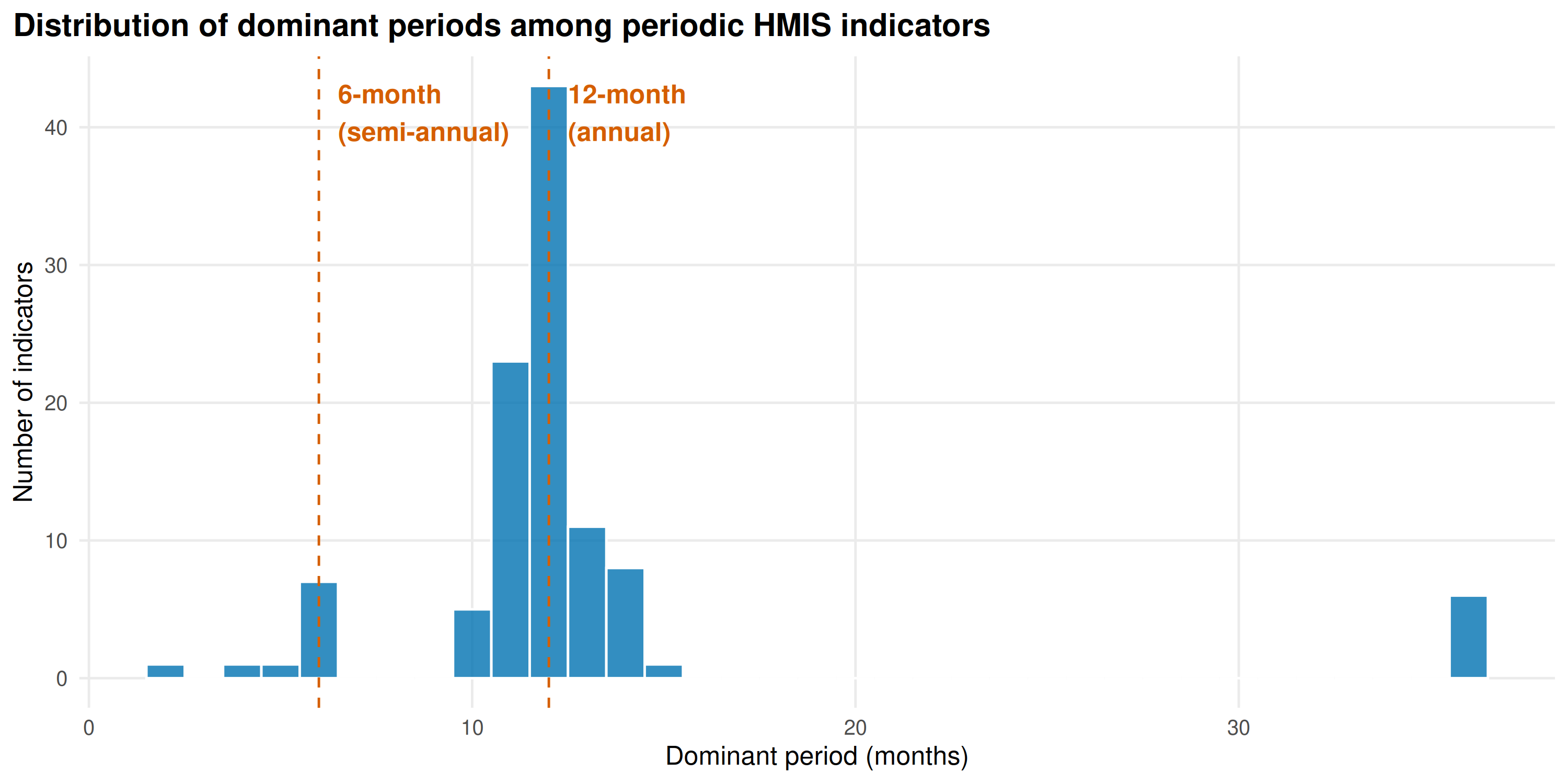
Cycle length distribution among periodic indicators:

periodic <- scan_results |> filter(is_periodic)

ggplot(periodic, aes(dominant_period)) +
  geom_histogram(binwidth = 1, fill = "#0072B2", color = "white", alpha = 0.8) +
  geom_vline(xintercept = c(6, 12), linetype = "dashed", color = "#D55E00") +
  annotate("text",
    x = 12.5, y = Inf, label = "12-month\n(annual)",
    hjust = 0, vjust = 1.5, color = "#D55E00", fontface = "bold"
  ) +
  annotate("text",
    x = 6.5, y = Inf, label = "6-month\n(semi-annual)",
    hjust = 0, vjust = 1.5, color = "#D55E00", fontface = "bold"
  ) +
  labs(
    x = "Dominant period (months)",
    y = "Number of indicators",
    title = "Distribution of dominant periods among periodic HMIS indicators"
  ) +
  theme_minimal(base_size = 12) +
  theme(
    plot.title = element_text(face = "bold"),
    plot.title.position = "plot",
    panel.grid.minor = element_blank()
  )

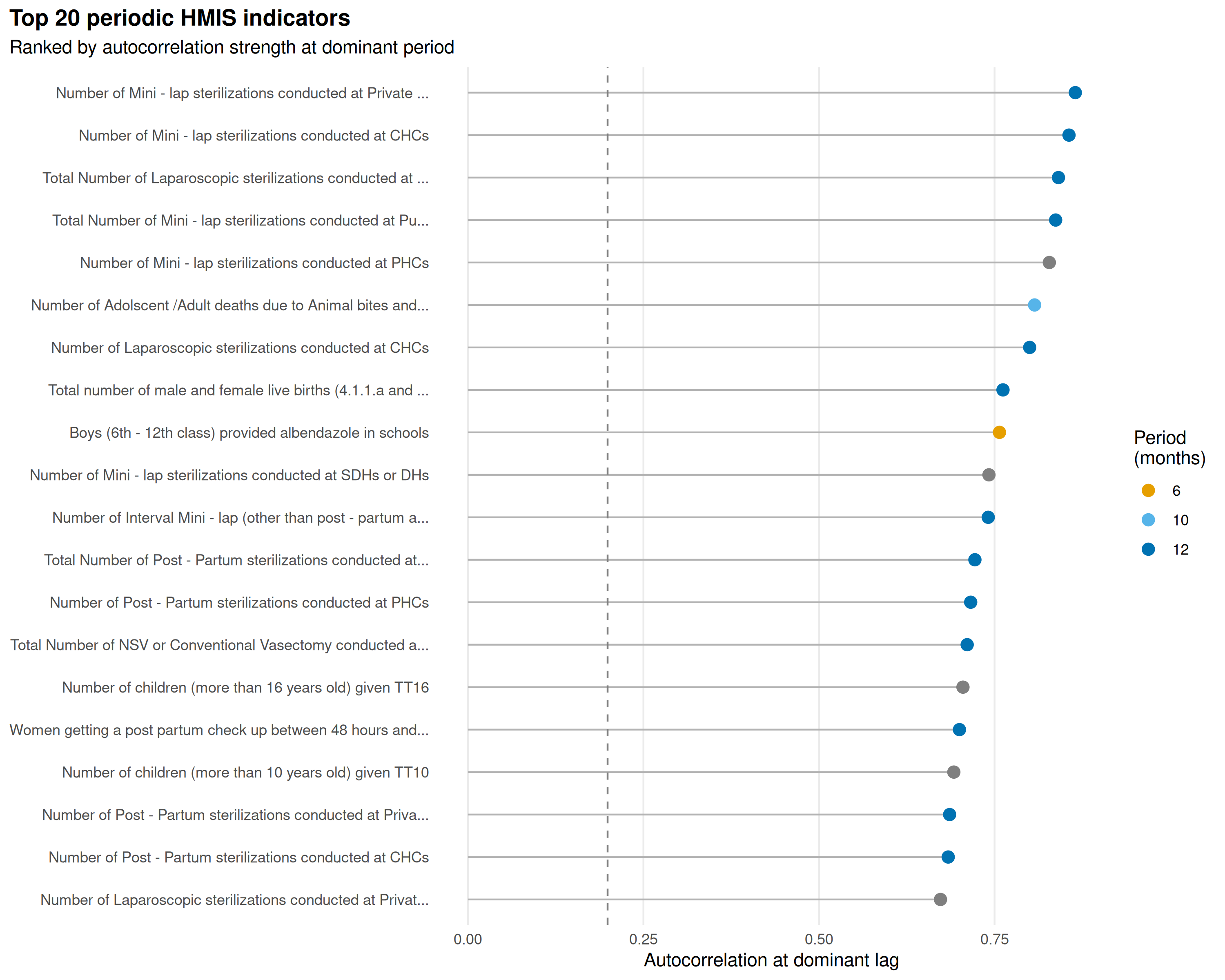
Strongest periodic signals

Top 20 indicators by autocorrelation at their dominant period:

top_periodic <- periodic |>
  arrange(desc(acf_peak)) |>
  head(20) |>
  mutate(
    short_name = ifelse(nchar(canonical_name) > 60,
      paste0(substr(canonical_name, 1, 57), "..."),
      canonical_name
    ),
    short_name = make.unique(short_name),
    short_name = factor(short_name, levels = rev(short_name))
  )

ggplot(top_periodic, aes(acf_peak, short_name)) +
  geom_segment(aes(xend = 0, yend = short_name), color = "grey70") +
  geom_point(aes(color = factor(round(dominant_period))), size = 3) +
  geom_vline(
    xintercept = scan_results$acf_threshold[1],
    linetype = "dashed", color = "grey50"
  ) +
  scale_color_manual(
    values = c(
      "6" = "#E69F00", "12" = "#0072B2", "3" = "#009E73",
      "4" = "#CC79A7", "9" = "#D55E00", "10" = "#56B4E9",
      "5" = "#F0E442", "8" = "#999999", "7" = "#D55E00"
    ),
    name = "Period\n(months)"
  ) +
  labs(
    x = "Autocorrelation at dominant lag",
    y = NULL,
    title = "Top 20 periodic HMIS indicators",
    subtitle = "Ranked by autocorrelation strength at dominant period"
  ) +
  theme_minimal(base_size = 11) +
  theme(
    plot.title = element_text(face = "bold"),
    plot.title.position = "plot",
    panel.grid.minor = element_blank(),
    panel.grid.major.y = element_blank()
  )

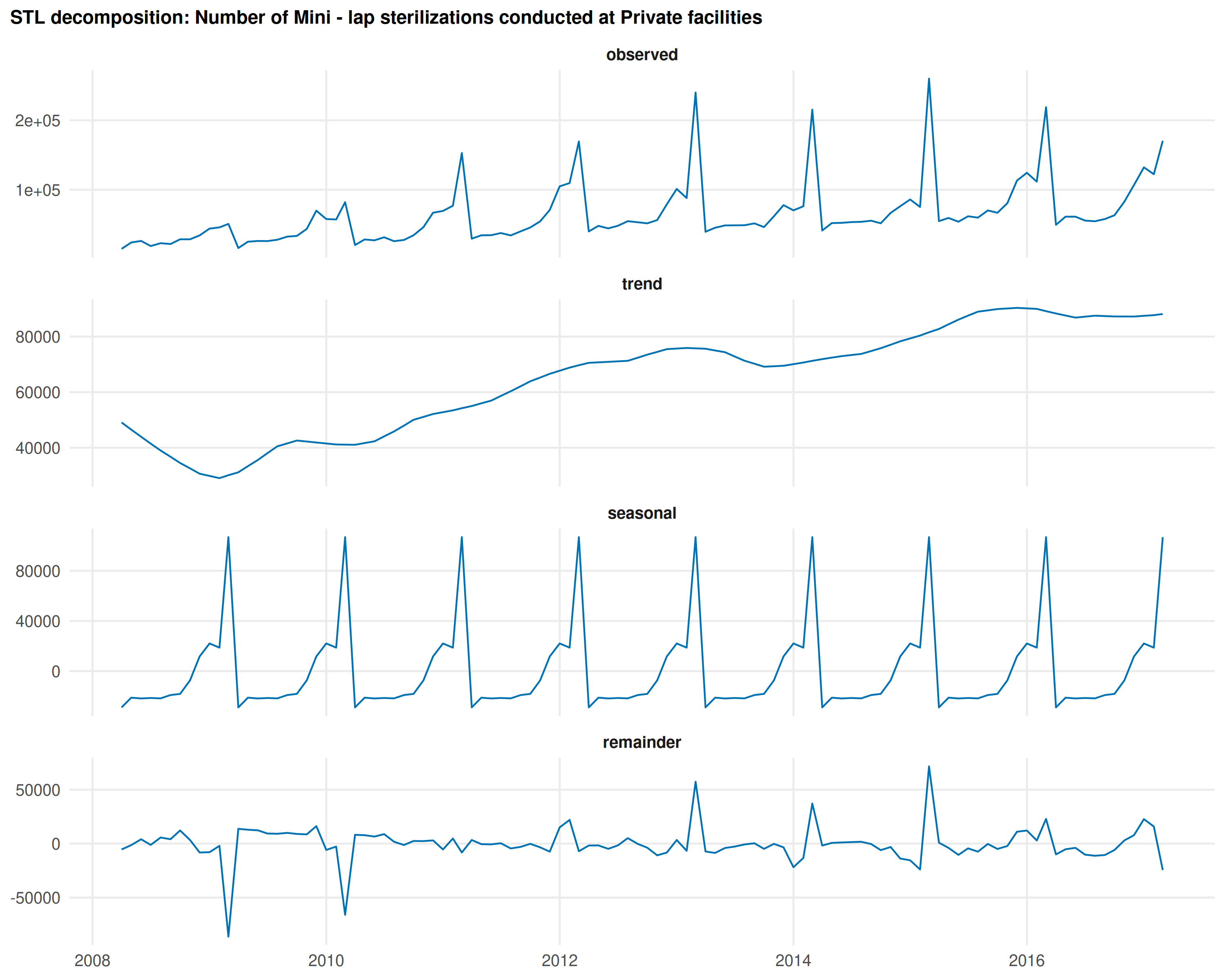
Decomposing the most seasonal indicator

top_name <- as.character(top_periodic$canonical_name[1])

national <- national_all |>
  filter(canonical_name == top_name)

decomp <- decompose_series(national)

decomp_long <- decomp |>
  pivot_longer(
    cols = c(observed, trend, seasonal, remainder),
    names_to = "component", values_to = "val"
  ) |>
  mutate(component = factor(component,
    levels = c("observed", "trend", "seasonal", "remainder")
  ))

ggplot(decomp_long, aes(date, val)) +
  geom_line(color = "#0072B2", linewidth = 0.5) +
  facet_wrap(~component, ncol = 1, scales = "free_y") +
  labs(
    x = NULL, y = NULL,
    title = paste("STL decomposition:", top_name)
  ) +
  theme_minimal(base_size = 12) +
  theme(
    strip.text = element_text(face = "bold"),
    panel.grid.minor = element_blank(),
    plot.title = element_text(face = "bold", size = 11),
    plot.title.position = "plot"
  )

All indicators: periodicity scores

All scanned indicators with periodicity results at the national level.

scan_results |>
  arrange(desc(is_periodic), desc(acf_peak)) |>
  dplyr::select(
    Indicator = canonical_name,
    Months = n_months,
    Periodic = is_periodic,
    `Period (months)` = dominant_period,
    `Spectral power (%)` = spectral_power_pct,
    `ACF peak` = acf_peak
  ) |>
  DT::datatable(
    filter = "top",
    options = list(pageLength = 20, scrollX = TRUE),
    rownames = FALSE
  )

Pre-computed seasonal indicators

hmis_seasonality is a bundled dataset of 129 indicators identified as strongly seasonal via harmonic regression and Kruskal-Wallis tests:

data(hmis_seasonality)

hmis_seasonality |>
  dplyr::select(
    canonical_name, category, seasonal_strength,
    dominant_period, peak_month, trough_month
  ) |>
  arrange(desc(seasonal_strength)) |>
  DT::datatable(
    filter = "top",
    options = list(pageLength = 15, scrollX = TRUE),
    rownames = FALSE
  )