# Define non-state entities and UTs
exclude_states <- c(
  "All India", "M/O Defence", "M/O Railways", "Chandigarh",
  "A & N Islands", "Andaman & Nicobar Islands", "Lakshadweep",
  "The Dadra And Nagar Haveli And Daman And Diu", "DNHDD",
    "Dadra & Nagar Haveli and Daman & Diu",
  "Jammu And Kashmir", "Jammu & Kashmir",
  "Ladakh", "Puducherry", "Goa", "Telangana"
)

north_states <- c("Uttar Pradesh", "Bihar", "Punjab", "Haryana", "Rajasthan", "Madhya Pradesh", "Chandigarh")
north_eastern_states = c("Arunachal Pradesh", "Assam", "Manipur", "West Bengal", "Jharkhand", "Sikkim")
south_states <- c("Andhra Pradesh", "Telangana", "Karnataka", "Kerala", "Tamil Nadu")
All cause-specific neonatal deaths
Indicator coverage
Cause Period Asphyxia 2008–2025 Sepsis 2008–2025 LBW 2008–2017 Prematurity 2023–2025 Others 2008–2025
Live births
births_old <- get_hmis(
  "Total number of male and female live births",
  sector = "Total",
  to     = "Mar 2017"
) |> add_calendar_vars()

births_new <- bind_rows(
  get_hmis("Number of male live births",   sector = "Total", from = "Apr 2017"),
  get_hmis("Number of female live births", sector = "Total", from = "Apr 2017")
) |> add_calendar_vars()

b_collapsed <- bind_rows(births_old, births_new) |>
  filter(!state %in% exclude_states) |>
  group_by(state, monyear, cal_year, month, month_num) |>
  summarise(births = sum(as.numeric(value), na.rm = TRUE), .groups = "drop")
Asphyxia
# Asphyxia: Apr 2008–Mar 2017 (old, 24hr–4wk) + Apr 2017–Apr 2025 (new, 0–4wk)
nmr_asphyxia <- bind_rows(
  get_hmis(
    "Number of cases of Infant deaths 24 hours to 4 weeks of birth with the probable cause being Asphyxia",
    sector   = "Total",
    category = "Total",
    to       = "Mar 2017"
  ),
  get_hmis(
    "Infant Deaths up to 4 weeks due to Asphyxia",
    sector = "Total",
    from   = "Apr 2017"
  )
) |>
  add_calendar_vars() |>
  group_by(state, monyear, cal_year, month, month_num) |>
  summarise(deaths = sum(as.numeric(value), na.rm = TRUE), .groups = "drop") |>
  inner_join(b_collapsed,
             by = c("state", "monyear", "cal_year", "month", "month_num")) |>
  mutate(nmr = (deaths / births) * 1000, cause = "Asphyxia")
Sepsis
Neonatal sepsis, a systemic infection in the first 28 days of life, encompasses bloodstream infections, meningitis, and pneumonia.
# Sepsis: Apr 2008–Mar 2017 (old) + Apr 2017–Apr 2025 (new)
nmr_sepsis <- bind_rows(
  get_hmis(
    "Number of cases of Infant deaths 24 hours to 4 weeks of birth with the probable cause being Sepsis",
    sector   = "Total",
    category = "Total",
    to       = "Mar 2017"
  ),
  get_hmis(
    "Infant Deaths up to 4 weeks due to Sepsis",
    sector = "Total",
    from   = "Apr 2017"
  )
) |>
  add_calendar_vars() |>
  group_by(state, monyear, cal_year, month, month_num) |>
  summarise(deaths = sum(as.numeric(value), na.rm = TRUE), .groups = "drop") |>
  inner_join(b_collapsed,
             by = c("state", "monyear", "cal_year", "month", "month_num")) |>
  mutate(nmr = (deaths / births) * 1000, cause = "Sepsis")
LBW
# LBW: Apr 2008–Mar 2017 only (dropped from new series)
nmr_lbw <- get_hmis(
  "Number of cases of Infant deaths 24 hours to 4 weeks of birth with the probable cause being LBW",
  sector   = "Total",
  category = "Total",
  to       = "Mar 2017"
) |>
  add_calendar_vars() |>
  group_by(state, monyear, cal_year, month, month_num) |>
  summarise(deaths = sum(as.numeric(value), na.rm = TRUE), .groups = "drop") |>
  inner_join(b_collapsed,
             by = c("state", "monyear", "cal_year", "month", "month_num")) |>
  mutate(nmr = (deaths / births) * 1000, cause = "LBW")

# Other: Apr 2008–Mar 2017 (old) + Apr 2017–Apr 2025 (new)
nmr_other <- bind_rows(
  get_hmis(
    "Number of cases of Infant deaths 24 hours to 4 weeks of birth with the probable cause being other than Sepsis, Asphyxia and LBW",
    sector   = "Total",
    category = "Total",
    to       = "Mar 2017"
  ),
  get_hmis(
    "Infant Deaths up to 4 weeks due to Other causes",
    sector = "Total",
    from   = "Apr 2017"
  )
) |>
  add_calendar_vars() |>
  group_by(state, monyear, cal_year, month, month_num) |>
  summarise(deaths = sum(as.numeric(value), na.rm = TRUE), .groups = "drop") |>
  inner_join(b_collapsed,
             by = c("state", "monyear", "cal_year", "month", "month_num")) |>
  mutate(nmr = (deaths / births) * 1000, cause = "Other")
# Prematurity: Apr 2023–Apr 2025 only
nmr_prematurity <- get_hmis(
  "Neonatal Deaths up to 4 weeks due to complications of Prematurity",
  sector = "Total",
  from   = "Apr 2023"
) |>
  add_calendar_vars() |>
  group_by(state, monyear, cal_year, month, month_num) |>
  summarise(deaths = sum(as.numeric(value), na.rm = TRUE), .groups = "drop") |>
  inner_join(b_collapsed,
             by = c("state", "monyear", "cal_year", "month", "month_num")) |>
mutate(nmr = (deaths / births) * 1000, cause = "Prematurity")Ratio Attribution Calibration: Scaling Factor for Indicator Alignment
In April 2017, HMIS indicators for neonatal death causes transitioned from reporting deaths occurring between 24 hours and 4 weeks to including all deaths from 0 to 4 weeks.
Assumption: The proportion of 0-4 week deaths occurring in the first 24 hours is stable over time — specifically that the Apr 2017–Mar 2023 fraction applies to 2008–2017 data.
Calculate the State & Cause specific Multipliers
deaths_24hr_old <- get_hmis(
  "Number of cases of Infant deaths within 24 hrs of birth",
  sector = "Total",
  to     = "Mar 2017"
) |> add_calendar_vars()

# from Apr 2017
deaths_24hr_new <- get_hmis(
  "Infant deaths within 24 hours (1 to 23 hours) of birth",
  sector = "Total",
  from   = "Apr 2017",
  to     = "Mar 2023"
) |> add_calendar_vars()
# get total 24hr deaths (from Apr 2017, no cause breakdown)
deaths_24hr_summarised <- deaths_24hr_new |>
  group_by(state, monyear, cal_year, month, month_num) |>
  summarise(deaths_24hr = sum(as.numeric(value), na.rm = TRUE),
            .groups = "drop")

# get total cause deaths (0-4 weeks)
# Total cause deaths post-2017 (denominator for frac_24hr)
deaths_cause_total <- bind_rows(
  nmr_asphyxia |> filter(cal_year >= 2017,
                          !(cal_year == 2017 & month_num <= 3)),
  nmr_sepsis   |> filter(cal_year >= 2017,
                          !(cal_year == 2017 & month_num <= 3)),
  nmr_other    |> filter(cal_year >= 2017,
                          !(cal_year == 2017 & month_num <= 3))
) |>
  group_by(state, monyear, cal_year, month, month_num) |>
  summarise(deaths_all_causes = sum(deaths, na.rm = TRUE), .groups = "drop")

# frac_24hr: mean fraction of 0-4wk deaths occurring in first 24hrs
# Computed from Apr 2017–Mar 2023 where 24hr indicator exists
frac_24hr <- deaths_24hr_summarised |>
  inner_join(deaths_cause_total,
             by = c("state", "monyear", "cal_year", "month", "month_num")) |>
  mutate(
    frac = deaths_24hr / deaths_all_causes,
    frac = pmin(pmax(frac, 0), 0.5)
  ) |>
  group_by(state) |>
  summarise(mean_frac_24hr = mean(frac, na.rm = TRUE), .groups = "drop")

# Apply calibration: scale up old series by 1/(1-frac_24hr)
all_causes_nmr_calibrated <- all_causes_nmr |>
  left_join(frac_24hr, by = "state") |>
  mutate(
    scale_factor = 1 / (1 - coalesce(mean_frac_24hr, 0.15)),
    # 0.15 fallback for states with no post-2017 24hr data
    nmr_adj = if_else(
      (cal_year < 2017 | (cal_year == 2017 & month_num <= 3)) &
        cause %in% c("Asphyxia", "Sepsis", "Other"),
      nmr * scale_factor,
      nmr
    )
  )
Seasonality across months | Normalized heatmaps
Min‑max normalization: highlights seasonal peaks relative to each state’s own range.
# Min-Max normalize calibrated NMR per state and cause
nmr_minmax_adj <- all_causes_nmr_calibrated |>
  # compute median adjusted NMR per state x cause x month across all years
  group_by(state, cause, month) |>
  summarise(med_nmr = median(nmr_adj, na.rm = TRUE), .groups = "drop") |>
  mutate(month = factor(month, levels = month.abb)) |>
  # normalize within each state x cause
  group_by(state, cause) |>
  mutate(
    s_min    = min(med_nmr,  na.rm = TRUE),
    s_max    = max(med_nmr,  na.rm = TRUE),
    nmr_norm = if_else(
      s_max > s_min,
      (med_nmr - s_min) / (s_max - s_min),
      0.5   # flat states -> mid-range
    )
  ) |>
  ungroup()

# Updated state ordering function for adjusted data
order_states_by_peak_adj <- function(df, cause_filter) {
  df |>
    filter(cause == cause_filter) |>
    group_by(state) |>
    slice_max(nmr_norm, n = 1, with_ties = FALSE) |>
    arrange(as.integer(month)) |>
    pull(state)
}

# Heatmap function for adjusted data
make_minmax_heatmap_adj <- function(cause_filter, title_label) {
  state_order <- order_states_by_peak_adj(nmr_minmax_adj, cause_filter)

  nmr_minmax_adj |>
    filter(cause == cause_filter) |>
    mutate(state = factor(state, levels = state_order)) |>
    ggplot(aes(x = month, y = state, fill = nmr_norm)) +
    geom_tile(color = "white", linewidth = 0.2) +
    scale_fill_distiller(
      palette   = "YlOrBr",
      direction = 1,
      name      = "Seasonal\nindex",
      limits    = c(0, 1)
    ) +
    labs(
      title    = paste0("Min-Max Normalized Adjusted NMR: ", title_label),
      caption = "States ordered by peak month",
      x = NULL, y = NULL
    ) +
    theme_hmis() +
    theme(
      panel.grid          = element_blank(),
      axis.text.x          = element_text(hjust = 1),
      axis.text          = element_text(face = "bold"),
      legend.position      = "top"
    ) +
    guides(
    fill = guide_colorbar(
      barwidth = 12,
      barheight = 0.55
    )
  ) +
  labs_hmis()
}

make_minmax_heatmap_adj("Asphyxia", "Asphyxia")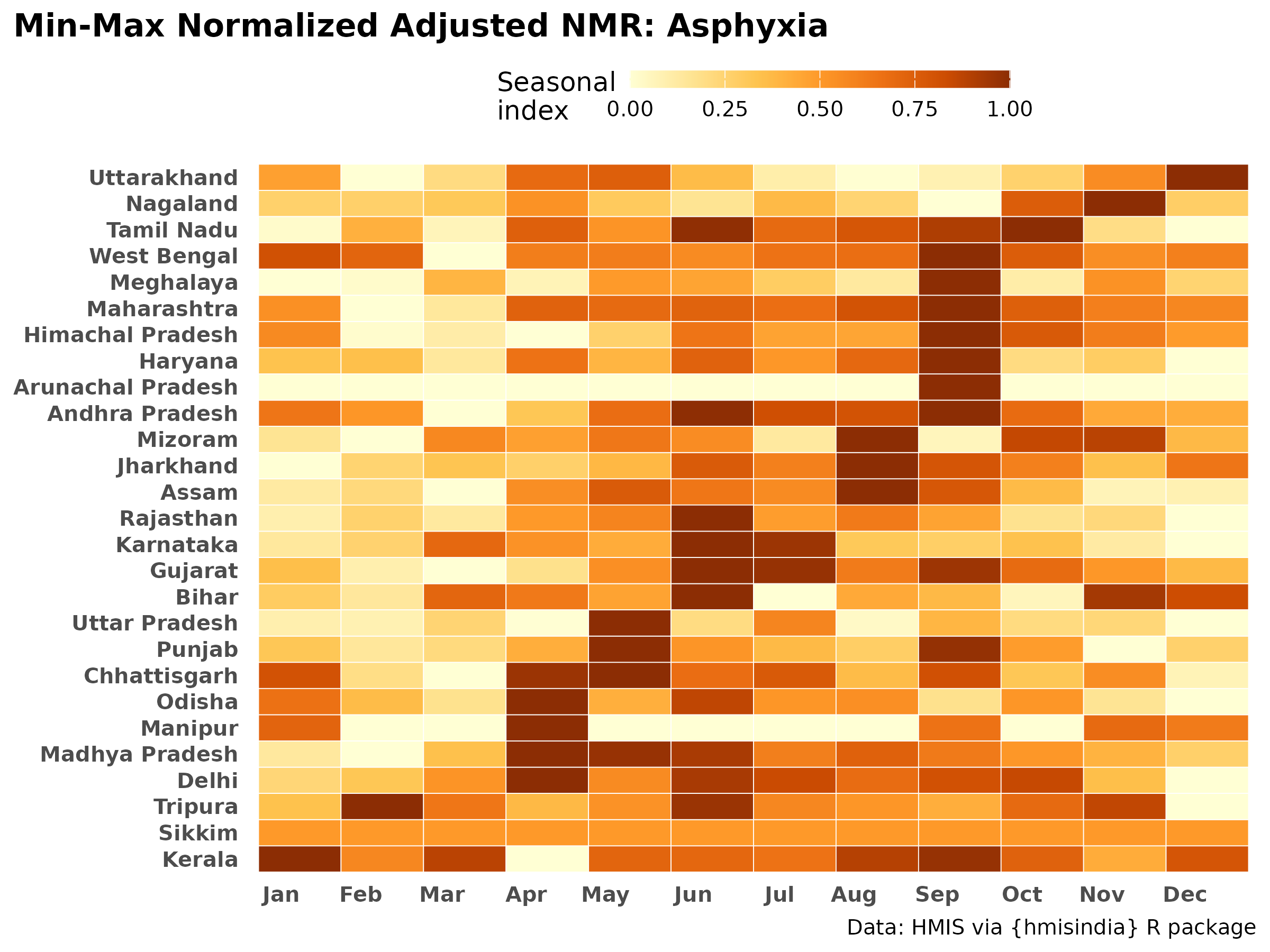
make_minmax_heatmap_adj("Sepsis", "Sepsis")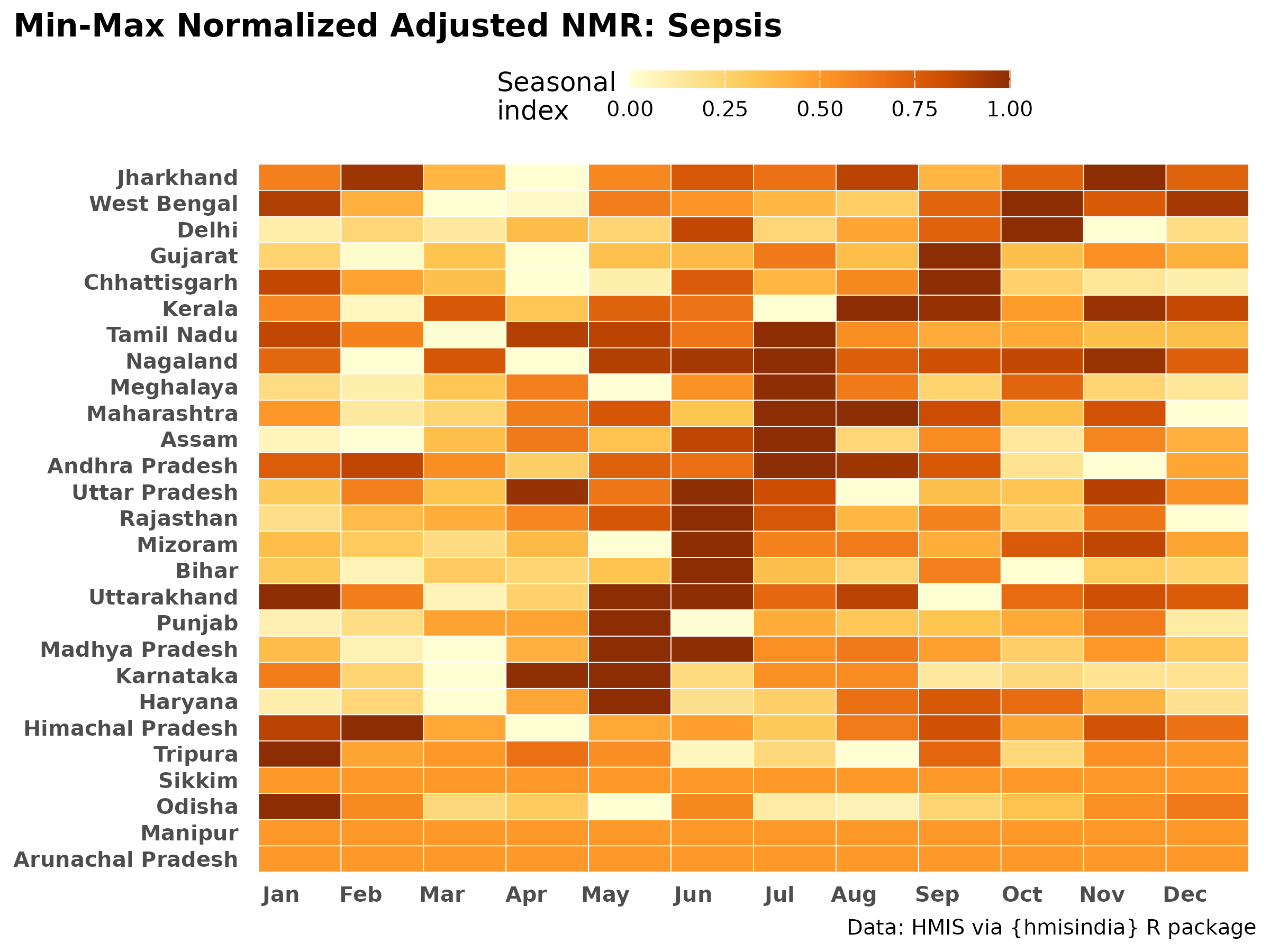
Z‑score normalization: highlights months unusually high/low compared to that state’s average
# Z-score normalize
nmr_zscore_adj <- all_causes_nmr_calibrated |>
  # Normalize within year first
  group_by(state, cause, cal_year) |>
  mutate(
    med_val = median(nmr_adj, na.rm = TRUE),
    mad_val = mad(nmr_adj,    na.rm = TRUE),
    z       = if_else(mad_val == 0, 0,
                      (nmr_adj - med_val) / mad_val)
  ) |>
  ungroup() |>
  # Cap at ±3
  mutate(z = pmin(pmax(z, -3), 3)) |>
  group_by(state, cause, month) |>
  summarise(med_z = median(z, na.rm = TRUE), .groups = "drop") |>
  mutate(month = factor(month, levels = month.abb))
# Asphyxia
ggplot(filter(nmr_zscore_adj, cause == "Asphyxia"),
       aes(x = month, y = state, fill = med_z)) +
  geom_tile(color = "white", linewidth = 0.1) +
        scale_fill_distiller(
      palette   = "PuOr",
      direction = 1
    ) +
    labs(title = "Z-score Normalized NMR: Asphyxia",
       x = NULL, y = NULL, fill = "Z-score") +
  theme_minimal() +
  theme(axis.text.x = element_text(hjust = 1),
              legend.position      = "top"
  ) +
    guides(
    fill = guide_colorbar(
      barwidth = 12,
      barheight = 0.55
    )
  ) +
  labs_hmis()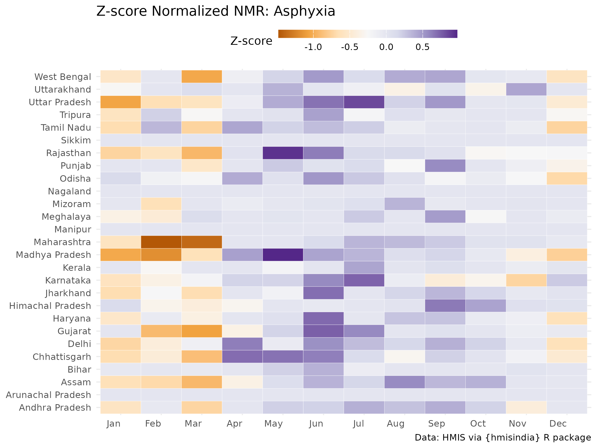
# Sepsis
ggplot(filter(nmr_zscore_adj, cause == "Sepsis"),
aes(x = month, y = state, fill = med_z)) +
geom_tile(color = "white", linewidth = 0.1) +
scale_fill_distiller(
palette = "PuOr",
direction = 1
) +
labs(title = "Z-score Normalized Adjusted NMR: Sepsis",
#subtitle = " ",
x = NULL, y = NULL, fill = "z-score") +
guides(
fill = guide_colorbar(
barwidth = 12,
barheight = 0.55
)
) +
theme_hmis() +
theme(axis.text = element_text(face = "bold"),
axis.text.x = element_text(hjust = 1),
legend.position = "top") +
labs_hmis()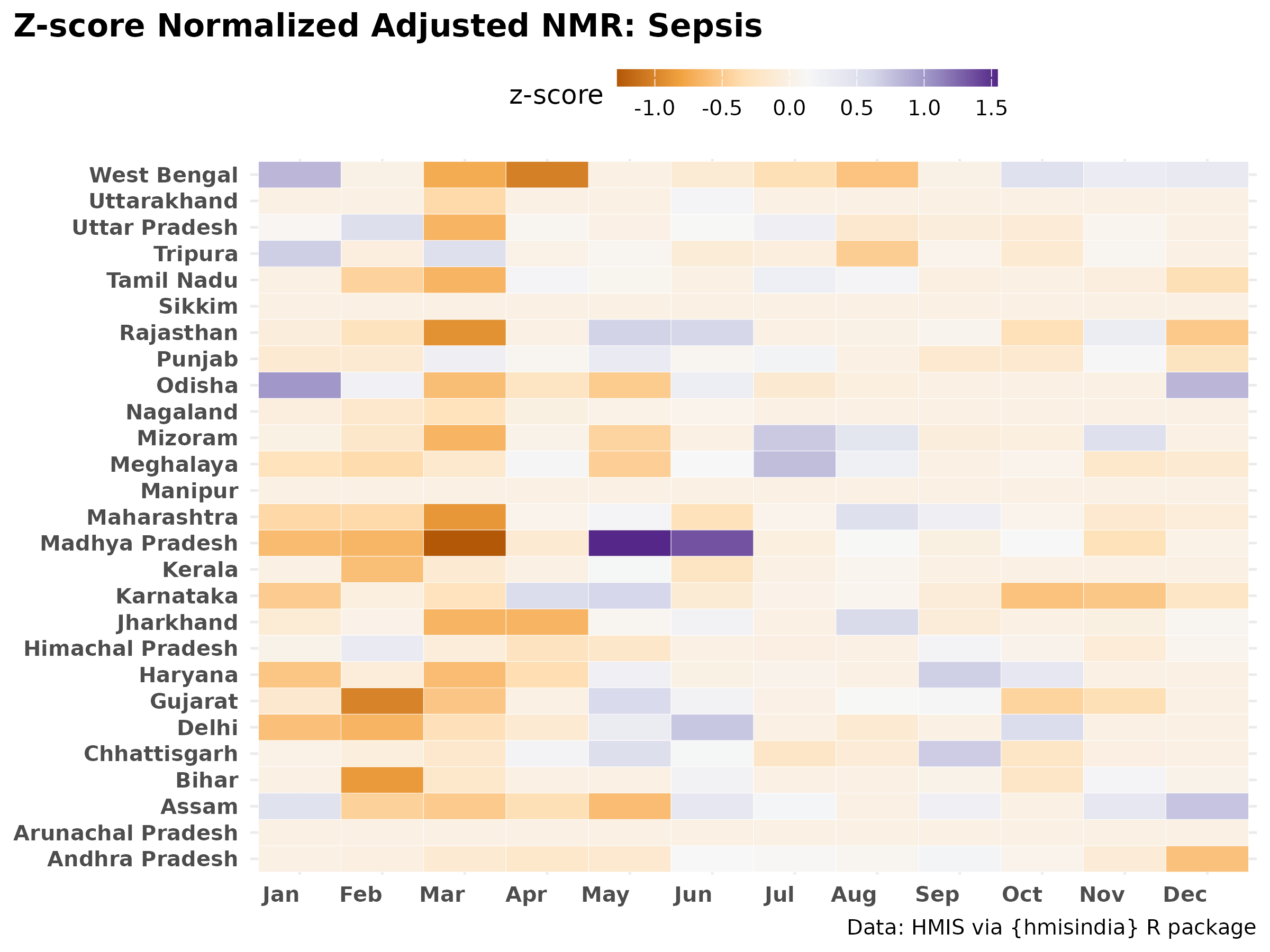 ## Is Asphyxia death correlated with Sepsis?
# Monthly median for Calibrated Asphyxia and Sepsis
cause_month_adj <- all_causes_nmr_calibrated %>%
  filter(cause %in% c("Asphyxia", "Sepsis")) %>%
  group_by(month, cal_year, cause) %>%
  summarise(median_nmr_adj = median(nmr_adj, na.rm = TRUE), .groups = "drop") %>%
  pivot_wider(names_from = cause, values_from = median_nmr_adj)

# Calibrated Correlation coefficient
cor_val_adj <- cor(cause_month_adj$Asphyxia, cause_month_adj$Sepsis, use = "complete.obs")
print(paste("Standard Correlation (Calibrated):", round(cor_val_adj, 3)))
#> [1] "Standard Correlation (Calibrated): 0.796"

#Current cor() on monthly medians pooled across all years.
#A partial correlation controlling for month would be more informative.
cor_data_adj <- cause_month_adj %>%
  mutate(month_num = match(month, month.abb)) %>%
  filter(!is.na(Asphyxia) & !is.na(Sepsis))

partial_res_adj <- pcor.test(cor_data_adj$Asphyxia, cor_data_adj$Sepsis, cor_data_adj$month_num)
print(paste("Partial Correlation (Calibrated):", round(partial_res_adj$estimate, 3)))
#> [1] "Partial Correlation (Calibrated): 0.795"
The partial correlation barely changed after controlling for month. This means the asphyxia-sepsis correlation is not just because both peak in monsoon together, but there might be state-level co-occurrence. States with high asphyxia tend to also have high sepsis regardless of month. This points to a common structural driver — likely healthcare system quality or SNCU capacity rather than a shared environmental exposure.
# Calibrated Monthly National Averages
seasonal_corr_adj <- all_causes_nmr_calibrated %>%
  filter(cause %in% c("Asphyxia", "Sepsis")) %>%
  group_by(month, cause) %>%
  summarise(med_nmr_adj = median(nmr_adj, na.rm = TRUE), .groups = "drop") %>%
  mutate(month = factor(month, levels = month.abb)) %>%
  arrange(cause, month) %>%
  group_by(cause) %>%
  mutate(rel_change_adj = (med_nmr_adj - lag(med_nmr_adj)) / lag(med_nmr_adj) * 100) %>%
  ungroup()
ggplot(seasonal_corr_adj, aes(x = month, y = rel_change_adj, group = cause, color = cause)) +
  geom_line(linewidth = 1) +
  geom_hline(yintercept = 0, linetype = "dotted", color = "grey40") +
  theme_minimal() +
scale_color_manual(values = c(
  "Asphyxia"    = "steelblue",
  "Sepsis"      = "tan3"
)) +
labs(
    title = "Calibrated Monthly Growth Rate: Asphyxia vs Sepsis",
    subtitle = "% Relative change in Adjusted NMR compared to previous month",
    y = "% Change from Previous Month",
    x = NULL) +
  theme_hmis() +
  theme(legend.position = "top",
        legend.title = element_blank(),
        axis.text = element_text(face = "bold")) +
  labs_hmis()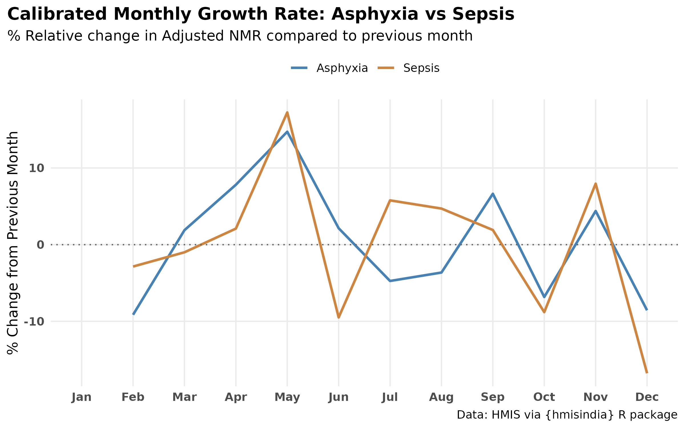
# Monthly averages for Calibrated Asphyxia and Sepsis
cause_month_adj_avg <- all_causes_nmr_calibrated %>%
  filter(cause %in% c("Asphyxia", "Sepsis")) %>%
  group_by(month, cal_year, cause) %>%
  summarise(avg_nmr_adj = mean(nmr_adj, na.rm = TRUE), .groups = "drop") %>%
  pivot_wider(names_from = cause, values_from = avg_nmr_adj)

# Calibrated Correlation coefficient (using Averages)
cor_val_adj_avg <- cor(cause_month_adj_avg$Asphyxia,
                       cause_month_adj_avg$Sepsis,
                       use = "complete.obs")

# % Relative change across month (National Averages)
seasonal_corr_adj_avg <- all_causes_nmr_calibrated %>%
  filter(cause %in% c("Asphyxia", "Sepsis")) %>%
  group_by(month, cause) %>%
  summarise(avg_nmr_adj = mean(nmr_adj, na.rm = TRUE), .groups = "drop") %>%
  mutate(month = factor(month, levels = month.abb)) %>%
  arrange(cause, month) %>%
  group_by(cause) %>%
  mutate(rel_change = (avg_nmr_adj - lag(avg_nmr_adj)) / lag(avg_nmr_adj) * 100) %>%
  ungroup() %>%
  filter(!is.na(rel_change))
# Plotting Calibrated Growth Rate
ggplot(seasonal_corr_adj_avg, aes(x = month, y = rel_change, group = cause, color = cause)) +
  geom_line(linewidth = 1) +
  geom_hline(yintercept = 0, linetype = "dotted", color = "grey40") +
  theme_minimal() +
  scale_color_manual(values = c("Asphyxia" = "steelblue4", "Sepsis" = "tan3")) +
  labs(
    title = "Calibrated Monthly Growth Rate: Asphyxia vs Sepsis",
    subtitle = "% Relative change in Adjusted NMR (National Average)",
    y = "% Change from Previous Month",
    x = NULL
  ) +
  theme_hmis() +
  theme(legend.position = "top",
            legend.title = element_blank(),
        axis.text = element_text(face = "bold")) +
  labs_hmis()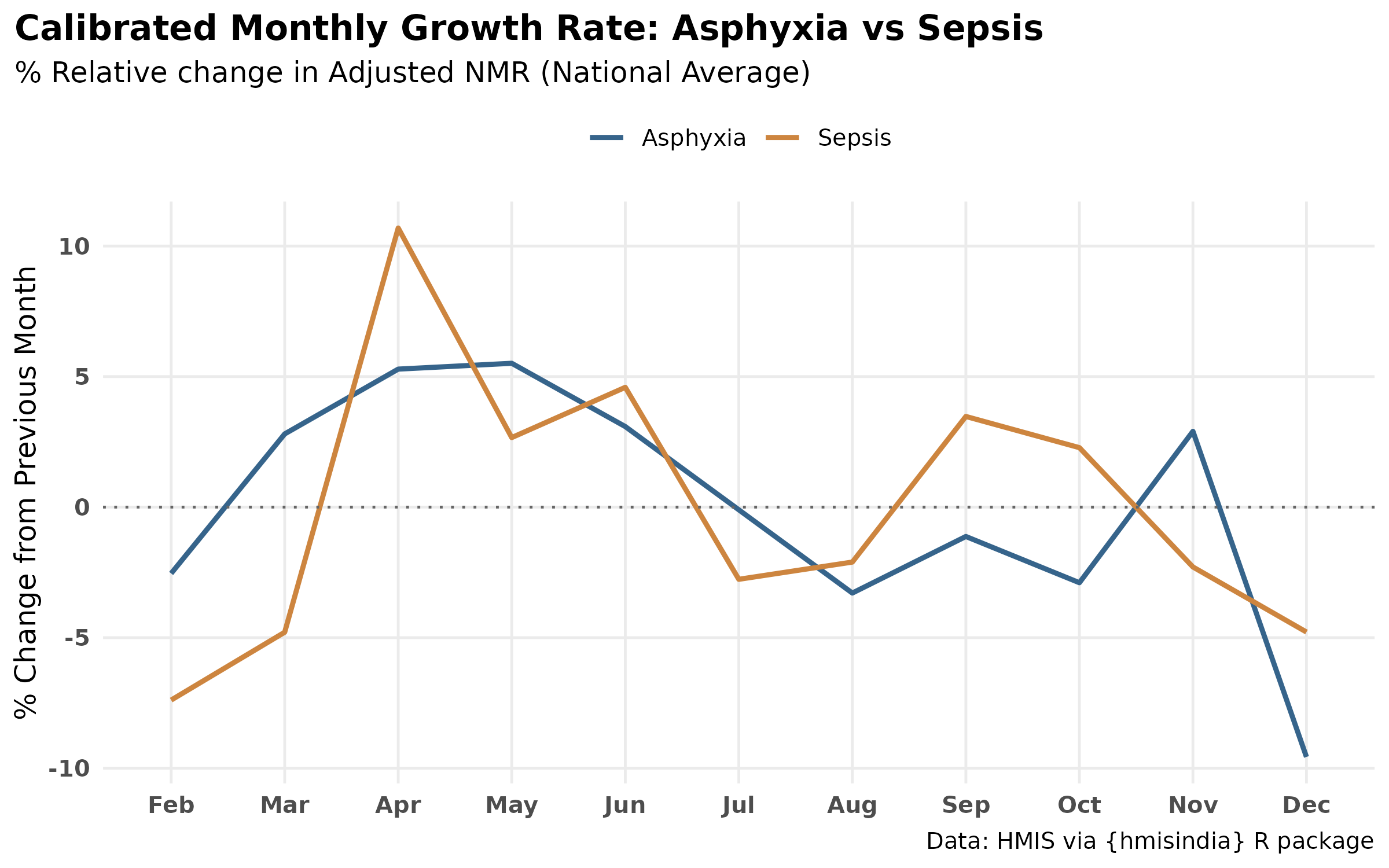
# National trend using calibrated NMR
national_trend_adj <- all_causes_nmr_calibrated %>%
  filter(cause %in% c("Asphyxia", "Sepsis", "LBW", "Other", "Prematurity")) %>%
  group_by(cal_year, cause) %>%
  summarise(national_med = median(nmr_adj, na.rm = TRUE), .groups = "drop")

ggplot(national_trend_adj, aes(x = cal_year, y = national_med, color = cause)) +
  geom_line(linewidth = 1) +
      geom_vline(xintercept = 2023, linetype = "dashed",
             color = "#E69F00", linewidth = 0.6) +
  annotate("text", x = 2023.1, y = Inf, vjust = 1.5, hjust = 0,
           label = "Prematurity\nadded", size = 2.8, color = "#E69F00") +
      geom_vline(xintercept = 2017, linetype = "dotted",
             color = "grey40", linewidth = 0.7) +
      annotate(geom = "text", x = 2015, y = 1.4,
           hjust = 0, size = 3, color = "grey4",
           label = "Apr 2017 indicator\nrename") +
scale_color_manual(values = c(
  "Asphyxia"    = "steelblue",
  "Sepsis"      = "tan3",
  "LBW"         = "#009E73",
  "Other"       = "#999999",
  "Prematurity" = "#E69F00"
)) +
    labs(
    title = "National NMR Trend",
    #subtitle = " ",
    y = "Adjusted NMR",
    x = NULL
  ) +
  theme_hmis() +
  theme(legend.position = "top",
            legend.title = element_blank(),
        axis.text = element_text(face = "bold")) +
  labs_hmis()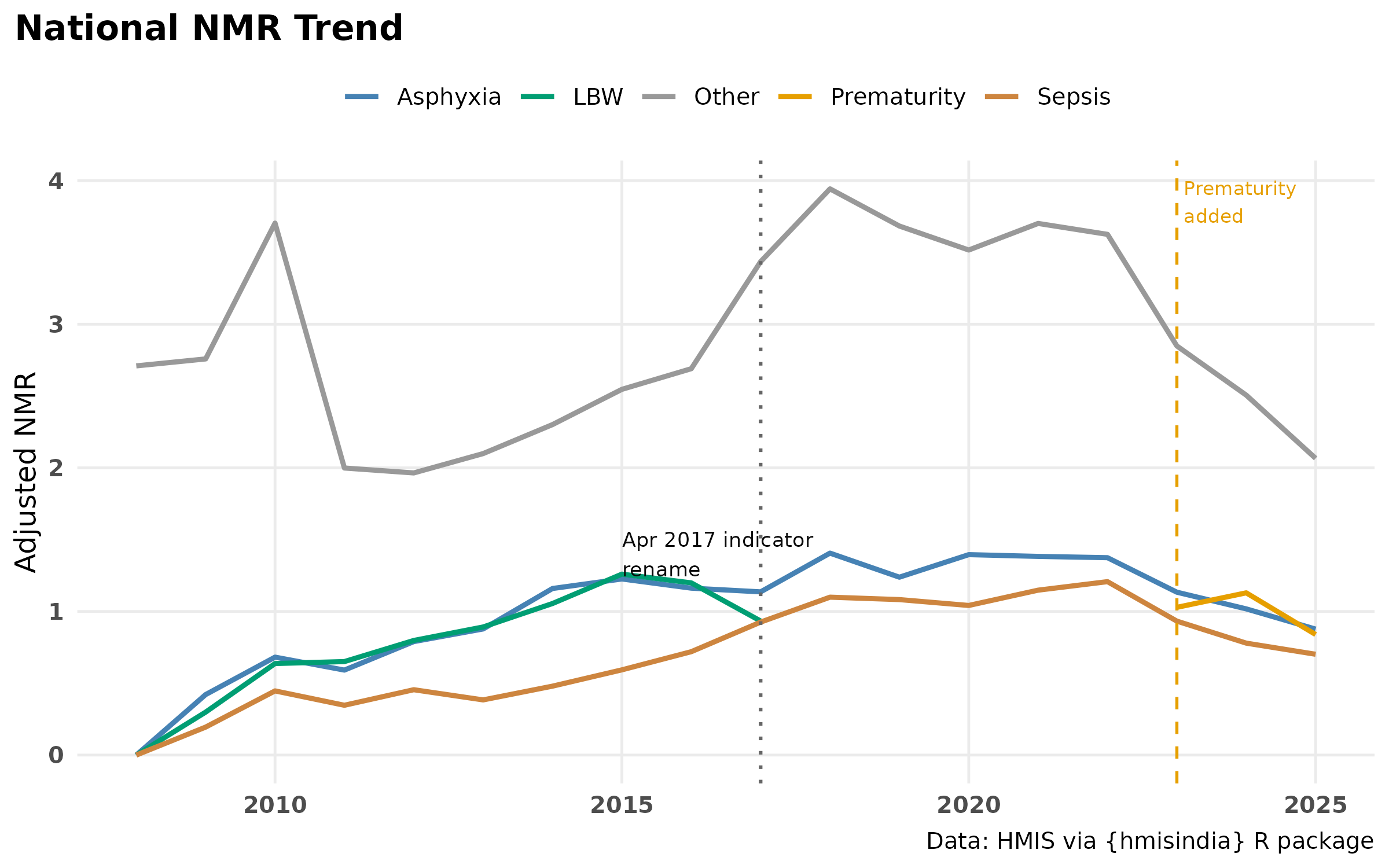
# lines starting from 0 in 2008, because the first year has incomplete data (Apr 2008 = start mid-year). Maybe filter out 2008
# State-level summary using calibrated NMR
cause_state_adj <- all_causes_nmr_calibrated |>
  group_by(state, cal_year, cause) |>
  summarise(avg_nmr_adj = mean(nmr_adj, na.rm = TRUE), .groups = "drop")

# Define high-burden list
high_burden <- c("Uttar Pradesh", "Bihar", "Assam", "West Bengal",
                 "Madhya Pradesh", "Chhattisgarh", "Jharkhand",
                 "Odisha", "Rajasthan")
# Faceted Asphyxia Trend
ggplot(filter(cause_state_adj, cause == "Asphyxia", state %in% high_burden),
       aes(x = cal_year, y = avg_nmr_adj)) +
  geom_line(color = "steelblue", linewidth = 0.6) +
    #geom_smooth(method = "loess", span = 0.2, color = "steelblue", se = FALSE) +
  facet_wrap(~state, scales = "free_y") +
  labs(
    title = "Asphyxia NMR: High-Burden States",
    #subtitle = "",
    y = "Adjusted NMR (per 1,000 live births)",
    x = NULL
  ) +
  theme_hmis() +
  labs_hmis()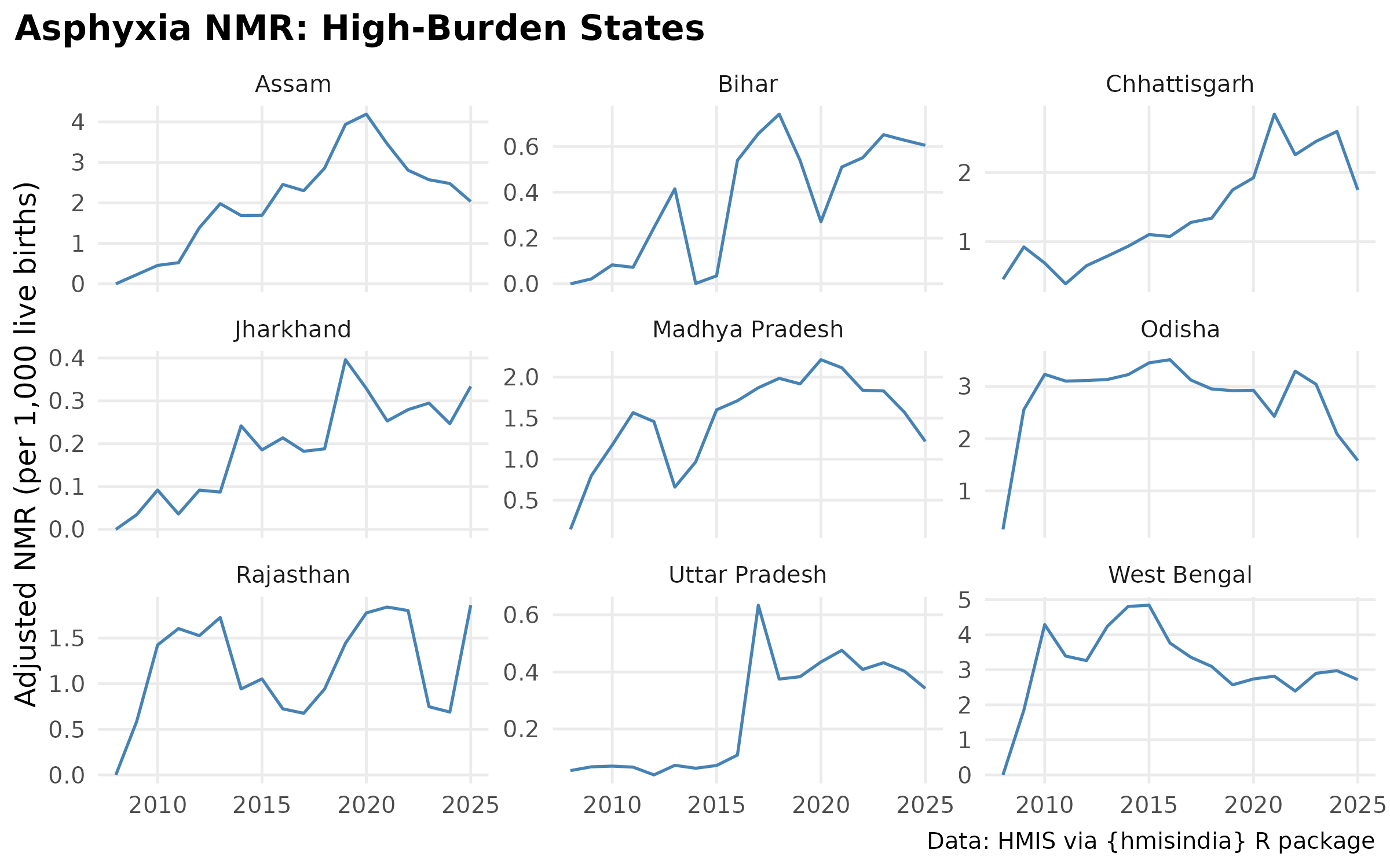
# Faceted Sepsis Trend
ggplot(filter(cause_state_adj, cause == "Sepsis", state %in% high_burden),
       aes(x = cal_year, y = avg_nmr_adj)) +
  geom_line(color = "tan3", linewidth = 0.6) +
  facet_wrap(~state, scales = "free_y") +
  labs(
    title = "Sepsis NMR: High-Burden States",
    #subtitle = "",
    y = "Adjusted NMR (per 1,000 live births)",
    x = NULL
  ) +
  theme_hmis() +
  labs_hmis()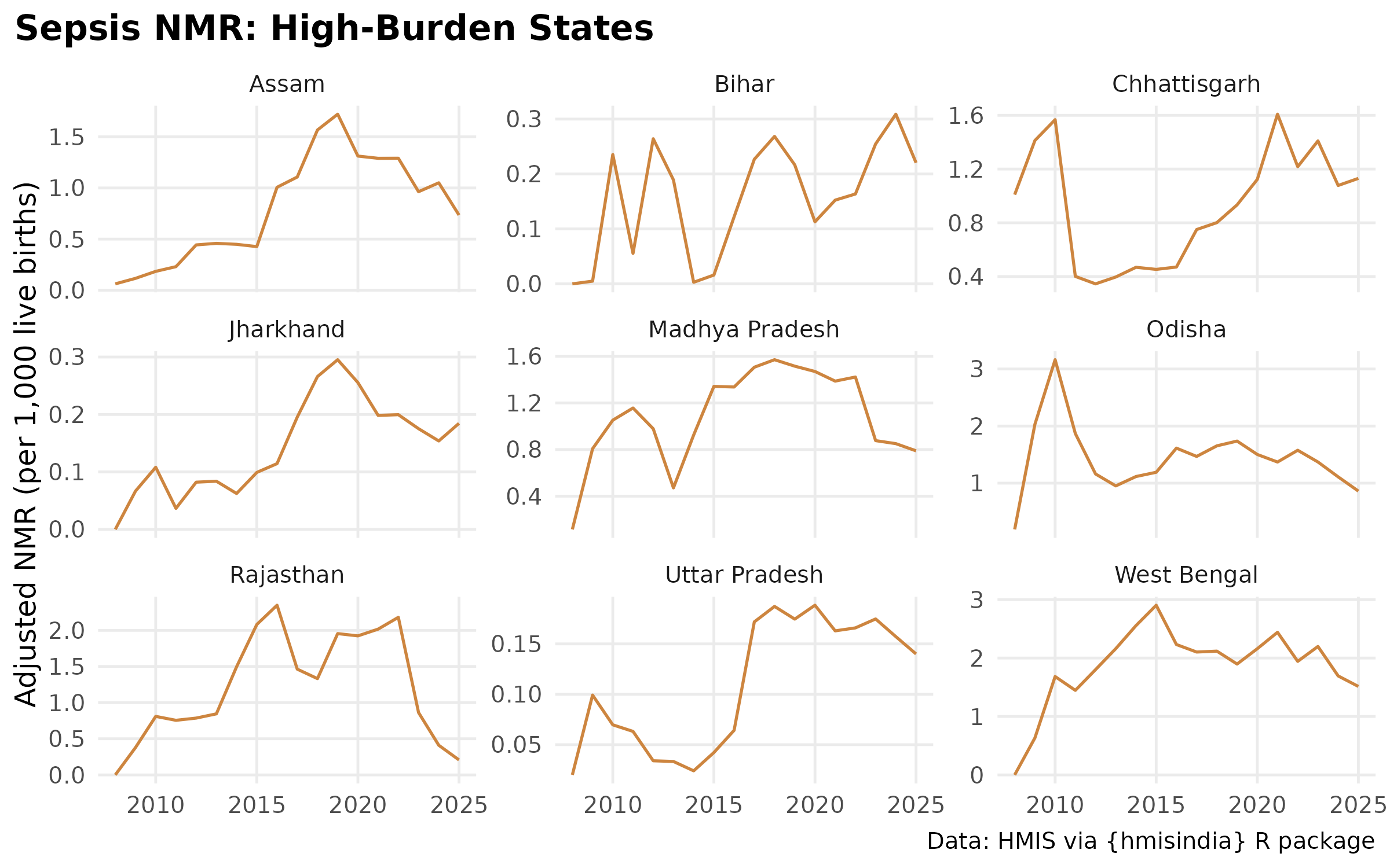
# lines starting from 0 in 2008, because the first year has incomplete data (Apr 2008 = start mid-year). Maybe filter out 2008
region_map <- data.frame(
  state = c(
    # North India
    "Uttar Pradesh", "Bihar", "Punjab", "Haryana", "Rajasthan", "Madhya Pradesh", "Chandigarh", "Uttarakhand", "Himachal Pradesh",
    # North Eastern India
    "Arunachal Pradesh", "Assam", "Manipur", "West Bengal", "Jharkhand", "Sikkim", "Meghalaya", "Mizoram", "Nagaland", "Tripura",
    # South India
    "Andhra Pradesh", "Telangana", "Karnataka", "Kerala", "Tamil Nadu",
    # West & Central
    "Maharashtra", "Gujarat", "Chhattisgarh", "Odisha"
  ),
  region = c(
    rep("North India", 9),
    rep("North East", 10),
    rep("South India", 5),
    rep("West/Central", 4)
  )
)

scatter_data_adj <- all_causes_nmr_calibrated |>
  filter(cause %in% c("Asphyxia", "Sepsis")) |>
  # Median adjusted NMR per state x month x cause
  group_by(state, month, cause) |>
  summarise(med_nmr_adj = median(nmr_adj, na.rm = TRUE), .groups = "drop") |>
  pivot_wider(names_from = cause, values_from = med_nmr_adj) |>
  left_join(region_map, by = "state") |>
  filter(!is.na(region), !is.na(Asphyxia), !is.na(Sepsis)) |>
  mutate(month = factor(month, levels = month.abb))
region_colours <- c(
  "North India"  = "#D55E00",
  "South India"  = "steelblue",
  "North East"     = "#009E73",
  "West/Central" = "#CC79A7"
)

ggplot(scatter_data_adj, aes(x = Asphyxia, y = Sepsis, color = region)) +
  coord_cartesian(xlim = c(0, 3.5), ylim = c(0, 2.5)) +
  geom_point(alpha = 0.5, size = 2.5) +
  geom_smooth(method = "lm", se = FALSE,
              color = "grey30", linewidth = 0.7, linetype = "dotted") +
  geom_abline(slope = 1, intercept = 0,
              linetype = "dashed", color = "grey70", linewidth = 0.5) +
  annotate("text", x = 0.3, y = 2.3, hjust = 0, size = 3.5,
           label = "r = 0.80 | partial r = 0.80\n(controlling for month)") +
  geom_text_repel(
    data = scatter_data_adj |>
      group_by(state) |>
      summarise(Asphyxia = median(Asphyxia), Sepsis = median(Sepsis)) |>
      left_join(region_map, by = "state"),
    aes(label = state),
    size = 3, fontface = "bold", max.overlaps = 15
  ) +
  scale_color_manual(values = region_colours, name = NULL) +
  labs(
    title   = "Asphyxia vs Sepsis NMR — State × Month combinations",
    x = "Asphyxia NMR (per 1,000 live births)",
    y = "Sepsis NMR (per 1,000 live births)"
  ) +
  theme_hmis() +
  theme(
    plot.title.position = "plot",
    panel.grid.minor    = element_blank(),
    legend.position     = "top"
  ) +
  labs_hmis()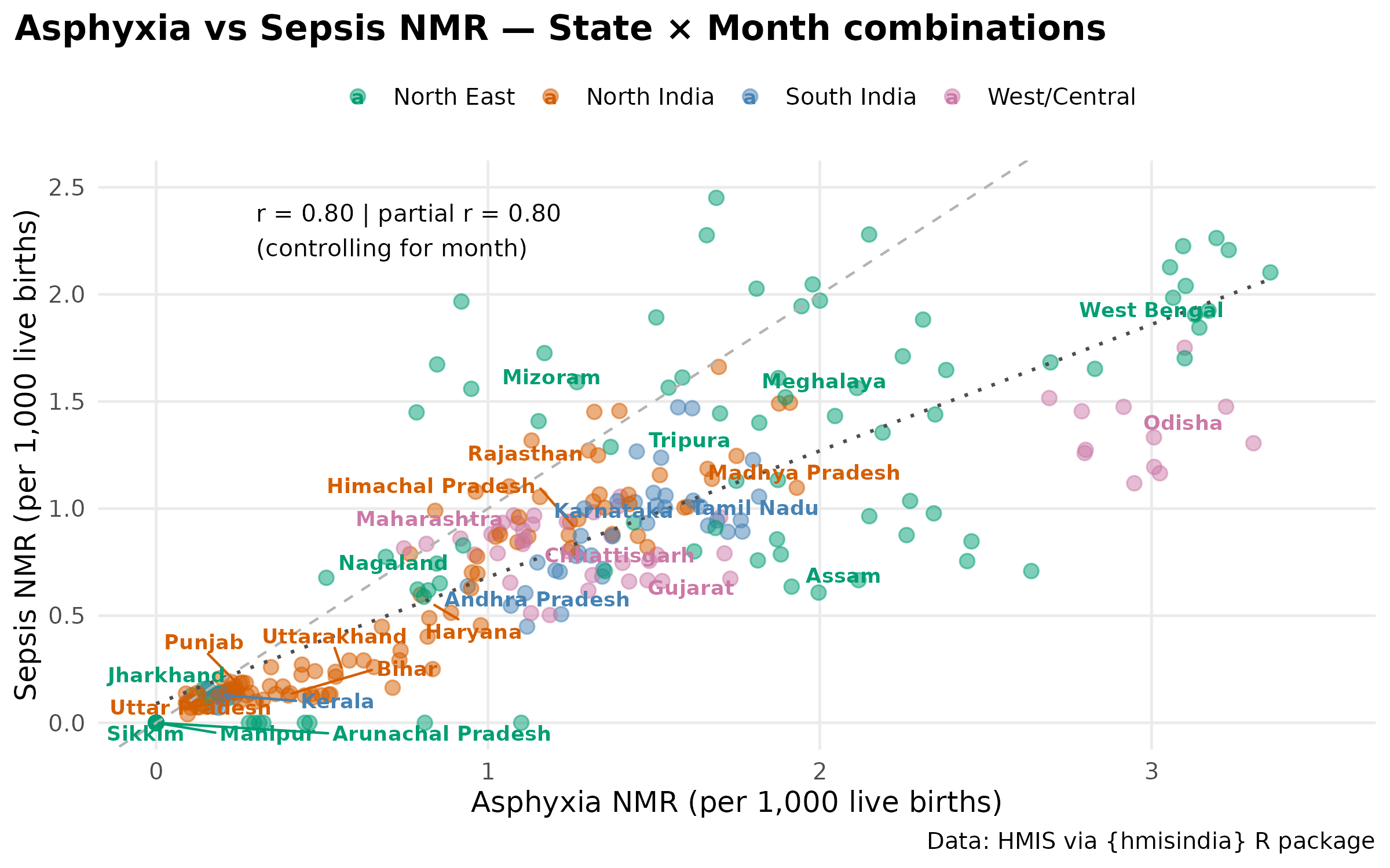
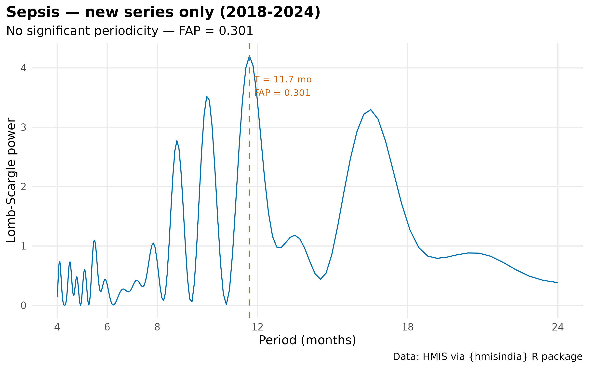
# Periodicity comparison: full series vs new series — by cause

causes_to_test <- c("Asphyxia", "Sepsis")

# Full series
periodicity_full <- all_causes_nmr_calibrated %>%
  filter(cause %in% causes_to_test) %>%
  group_by(monyear, cause) %>%
  summarise(nmr_adj = median(nmr_adj, na.rm = TRUE), .groups = "drop")

# New series only
periodicity_new <- all_causes_nmr_calibrated %>%
  filter(cause %in% causes_to_test,
         cal_year >= 2018, cal_year <= 2024) %>%
  group_by(monyear, cause) %>%
  summarise(nmr_adj = median(nmr_adj, na.rm = TRUE), .groups = "drop")

# Run for both series and both causes
results <- list()

for (s in c("full", "new")) {
  df <- if (s == "full") periodicity_full else periodicity_new
  for (cause_name in causes_to_test) {
    res <- detect_periodicity_ls(
      df %>% filter(cause == cause_name),
      value_col  = "nmr_adj",
      time_col   = "monyear",
      detrend    = TRUE,
      period_max = 24
    )
    results[[paste(cause_name, s, sep = "_")]] <- list(
      cause      = cause_name,
      series     = s,
      periodic   = res$is_periodic,
      period     = round(res$dominant_period, 1),
      fap        = signif(res$fap, 3),
      peak_power = round(res$peak_power, 2),
      result     = res
    )
  }
}

# Summary table
results_df <- purrr::map_dfr(results, function(r) {
  tibble(
    cause    = r$cause,
    series   = r$series,
    periodic = r$periodic,
    period   = r$period,
    fap      = r$fap,
    power    = r$peak_power
  )
}) |>
  mutate(series = if_else(series == "full",
                           "Full (2008-2025)",
                           "New only (2018-2024)")) |>
  arrange(cause, series)

print(results_df)
#> # A tibble: 4 × 6
#>   cause    series               periodic period    fap power
#>   <chr>    <chr>                <lgl>     <dbl>  <dbl> <dbl>
#> 1 Asphyxia Full (2008-2025)     FALSE      11.9 0.102   6.38
#> 2 Asphyxia New only (2018-2024) TRUE       11.8 0.0332  6.63
#> 3 Sepsis   Full (2008-2025)     FALSE      11.9 0.0992  6.41
#> 4 Sepsis   New only (2018-2024) FALSE      11.7 0.301   4.2

# Plot all four periodograms
plot(results[["Asphyxia_full"]]$result) +
  labs(title = "Asphyxia — full series (2008-2025)") +
  theme_hmis() + labs_hmis()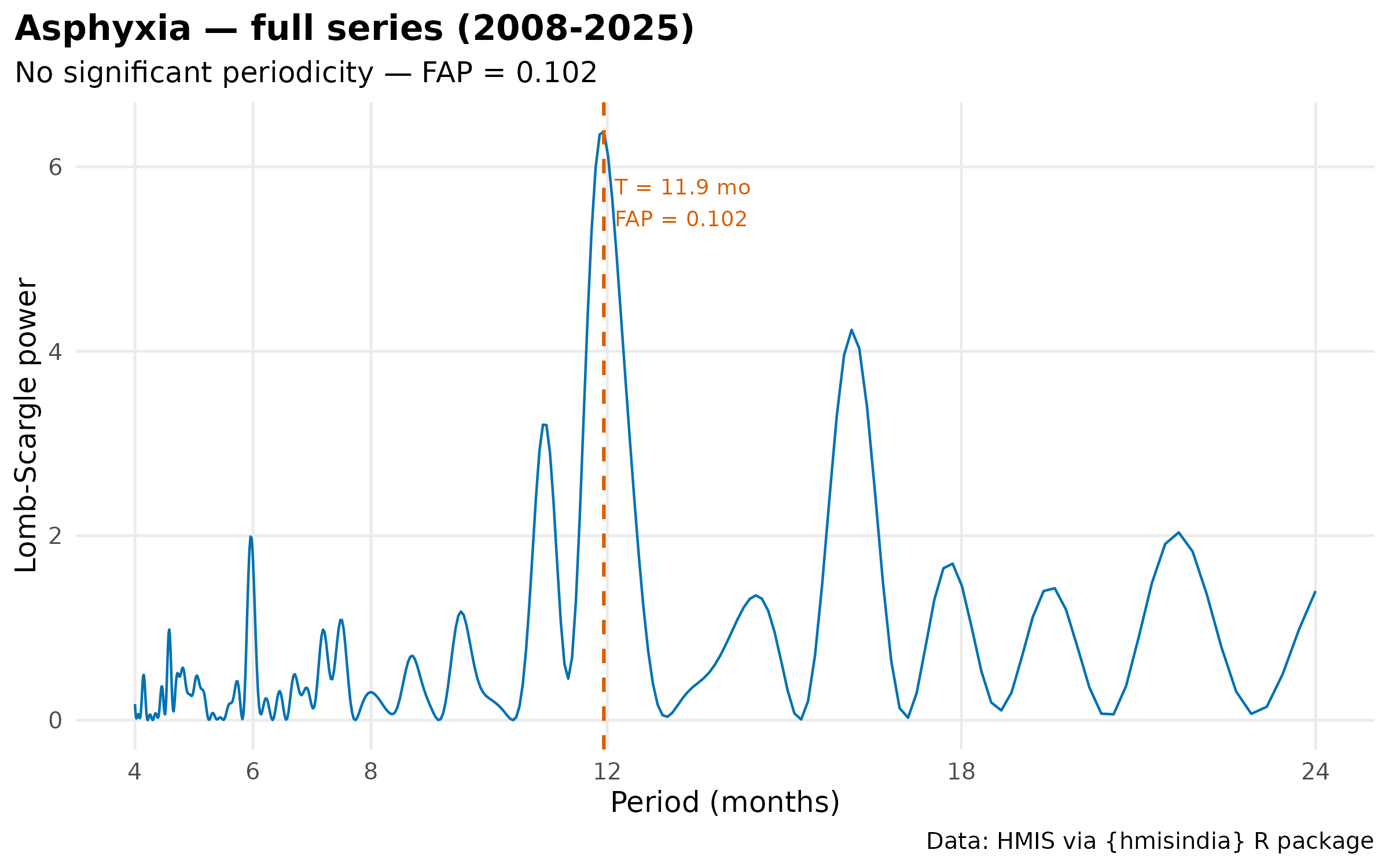
plot(results[["Asphyxia_new"]]$result) +
  labs(title = "Asphyxia — new series only (2018-2024)") +
  theme_hmis() + labs_hmis()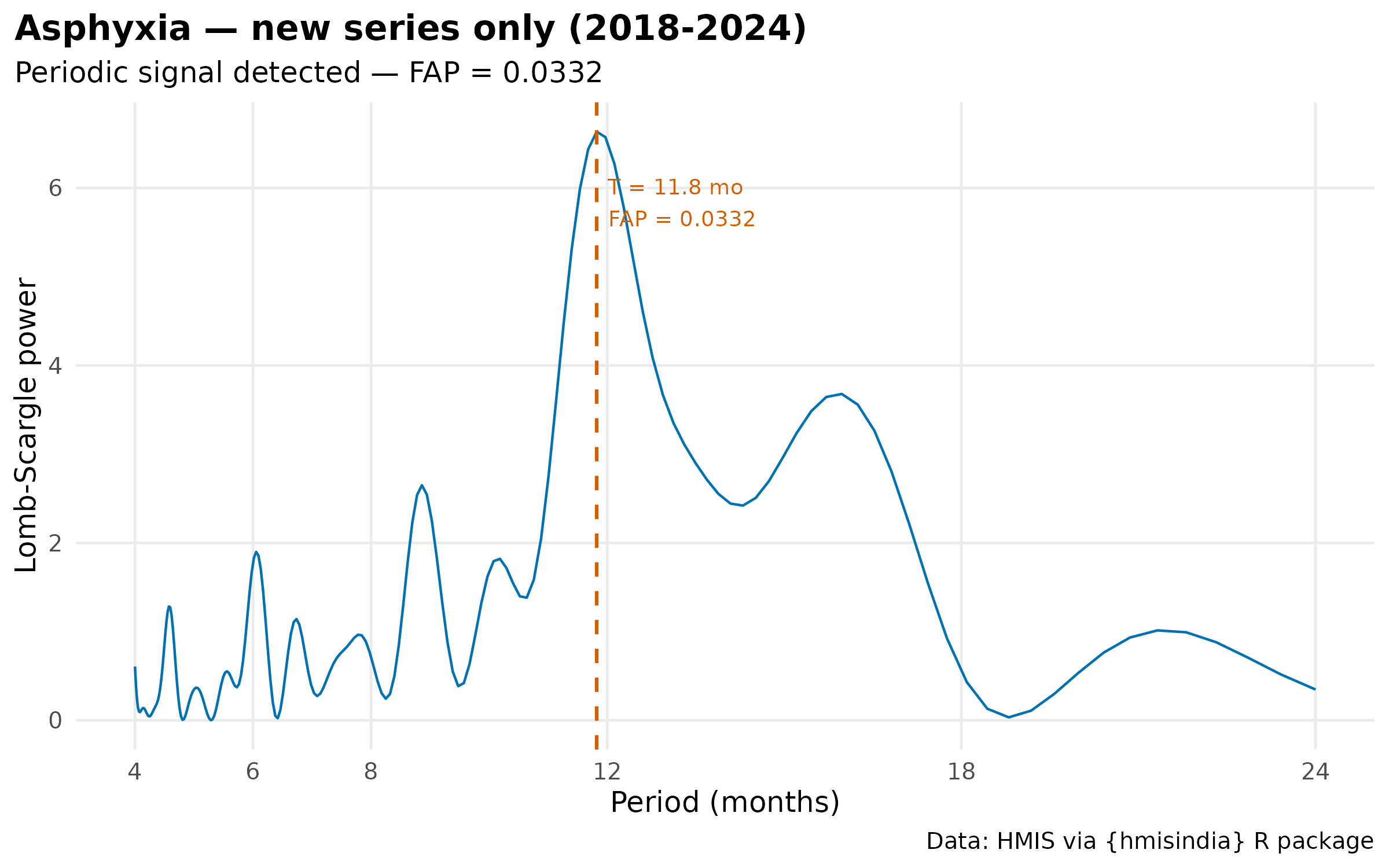
plot(results[["Sepsis_full"]]$result) +
  labs(title = "Sepsis — full series (2008-2025)") +
  theme_hmis() + labs_hmis()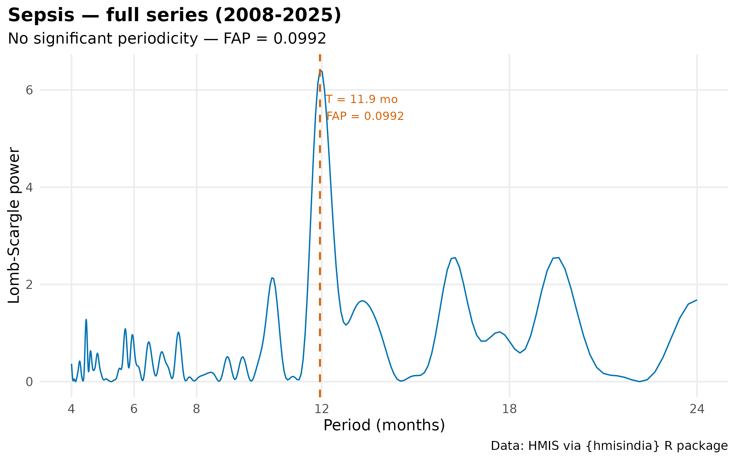
plot(results[["Sepsis_new"]]$result) +
  labs(title = "Sepsis — new series only (2018-2024)") +
  theme_hmis() + labs_hmis()