Malaria testing in India: trends, species, and diagnostics

library(hmisindia)
library(dplyr)
library(ggplot2)
library(tidyr)
library(DT)

data_available <- tryCatch(
  {
    pq <- hmisindia::get_parquet_path()
    nzchar(pq) && file.exists(pq)
  },
  error = function(e) FALSE
)
knitr::opts_chunk$set(eval = data_available)

HMIS reports monthly malaria surveillance from every state and union territory. We use test positivity rates (TPR = positives / tests) rather than raw case counts. A state that tests more will report more positives regardless of transmission.

From April 2017, HMIS splits malaria reporting into microscopy and RDT streams.

1. Total testing volume

Monthly blood smears examined for malaria since 2008:

smears <- get_hmis(
  "Number of blood smears examined for Malaria",
  category = "Total",
  sector = "Total"
)

national_smears <- smears |>
  mutate(date = parse_monyear(monyear)) |>
  group_by(date) |>
  summarise(total_smears = sum(value, na.rm = TRUE), .groups = "drop") |>
  arrange(date)

ggplot(national_smears, aes(date, total_smears / 1e6)) +
  geom_line(color = "#0072B2", linewidth = 0.8) +
  geom_smooth(
    method = "loess", span = 0.15, se = FALSE,
    color = "#D55E00", linewidth = 0.6, linetype = "dashed"
  ) +
  scale_x_date(date_labels = "%b %Y", date_breaks = "2 years") +
  scale_y_continuous(labels = scales::comma_format(suffix = "M")) +
  labs(
    x = NULL,
    y = "Blood smears examined (millions)",
    title = "National malaria testing volume, Apr 2008 - Dec 2024",
    subtitle = "Monthly blood smears examined across all states/UTs"
  ) +
  theme_minimal(base_size = 12) +
  theme(
    axis.text.x = element_text(angle = 45, hjust = 1),
    plot.title = element_text(face = "bold"),
    plot.title.position = "plot",
    panel.grid.minor = element_blank()
  )

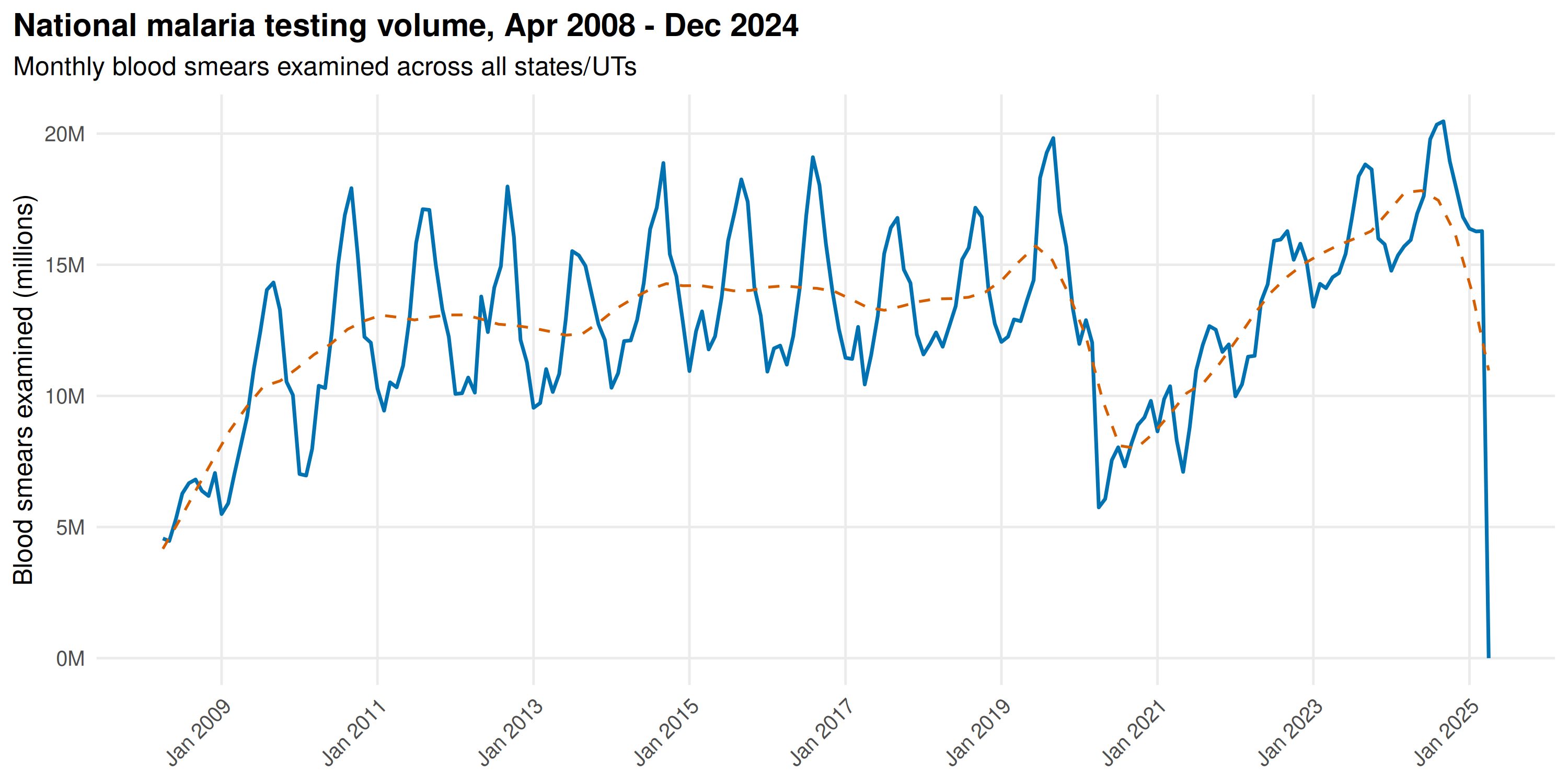
Testing volume grew from 2008 through the mid-2010s as the malaria elimination programme scaled up active surveillance. The early 2020 dip is the COVID-19 lockdown; routine field testing collapsed for several months. Volumes recovered by late 2020, but the gap likely masked true transmission during peak monsoon months.

plot_heatmap(
  smears,
  title = "Blood smears examined for malaria by state and month",
  legend_title = "Smears"
)

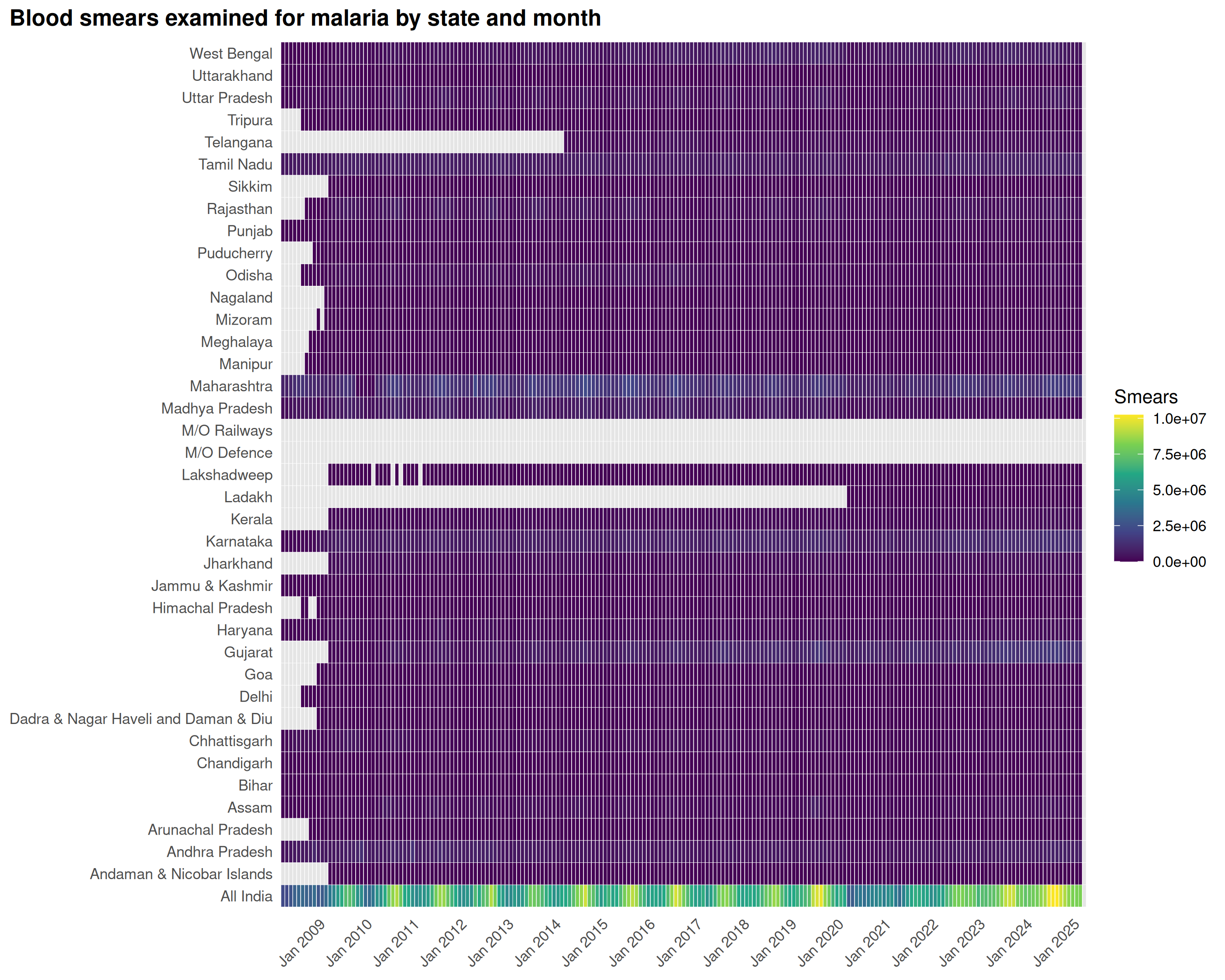
A handful of states (Odisha, Chhattisgarh, Jharkhand, Madhya Pradesh, Rajasthan) dominate testing volumes. Smaller states test few samples, making their positivity rates noisier.

2. Positivity rates as incidence

From April 2017, HMIS separates microscopy and RDT results.

vivax_micro <- get_hmis(
  "Malaria (Microscopy Tests) - Plasmodium Vivax test positive",
  category = "Total", sector = "Total",
  from = "Apr 2017", to = "Dec 2024"
)

falci_micro <- get_hmis(
  "Malaria (Microscopy Tests) - Plasmodium Falciparum test positive",
  category = "Total", sector = "Total",
  from = "Apr 2017", to = "Dec 2024"
)

# RDT positives (note the typo "Plamodium" in the original HMIS data)
falci_rdt <- get_hmis(
  "Malaria (RDT) - Plamodium Falciparum test positive",
  category = "Total", sector = "Total",
  from = "Apr 2017", to = "Dec 2024"
)

# Denominators
smears_post <- get_hmis(
  "Number of blood smears examined for Malaria",
  category = "Total", sector = "Total",
  from = "Apr 2017", to = "Dec 2024"
)

rdt_conducted <- get_hmis(
  "RDT conducted for Malaria",
  category = "Total", sector = "Total",
  from = "Apr 2017", to = "Dec 2024"
)

# Aggregate each indicator to national monthly totals
agg <- function(df, col_name) {
  df |>
    mutate(date = parse_monyear(monyear)) |>
    group_by(date) |>
    summarise(!!col_name := sum(value, na.rm = TRUE), .groups = "drop")
}

national_tpr <- agg(vivax_micro, "vivax_pos") |>
  inner_join(agg(falci_micro, "falci_pos"), by = "date") |>
  inner_join(agg(falci_rdt, "falci_rdt_pos"), by = "date") |>
  inner_join(agg(smears_post, "smears"), by = "date") |>
  inner_join(agg(rdt_conducted, "rdt_tests"), by = "date") |>
  mutate(
    tpr_vivax_micro    = vivax_pos / smears * 100,
    tpr_falci_micro    = falci_pos / smears * 100,
    tpr_falci_rdt      = falci_rdt_pos / rdt_tests * 100
  )

tpr_long <- national_tpr |>
  select(date, tpr_vivax_micro, tpr_falci_micro, tpr_falci_rdt) |>
  pivot_longer(-date, names_to = "test_type", values_to = "tpr") |>
  mutate(test_type = case_when(
    test_type == "tpr_vivax_micro" ~ "Vivax (Microscopy)",
    test_type == "tpr_falci_micro" ~ "Falciparum (Microscopy)",
    test_type == "tpr_falci_rdt" ~ "Falciparum (RDT)"
  ))

pal_tpr <- c(
  "Vivax (Microscopy)"      = "#E69F00",
  "Falciparum (Microscopy)" = "#0072B2",
  "Falciparum (RDT)"        = "#D55E00"
)

ggplot(tpr_long, aes(date, tpr, color = test_type)) +
  geom_line(linewidth = 0.8) +
  scale_color_manual(values = pal_tpr, name = "Test type") +
  scale_x_date(date_labels = "%b %Y", date_breaks = "1 year") +
  labs(
    x = NULL,
    y = "Test positivity rate (%)",
    title = "National malaria test positivity rates by species and diagnostic method",
    subtitle = "Post-2017 period (Apr 2017 - Dec 2024)"
  ) +
  theme_minimal(base_size = 12) +
  theme(
    axis.text.x = element_text(angle = 45, hjust = 1),
    plot.title = element_text(face = "bold"),
    plot.title.position = "plot",
    panel.grid.minor = element_blank(),
    legend.position = "bottom"
  )

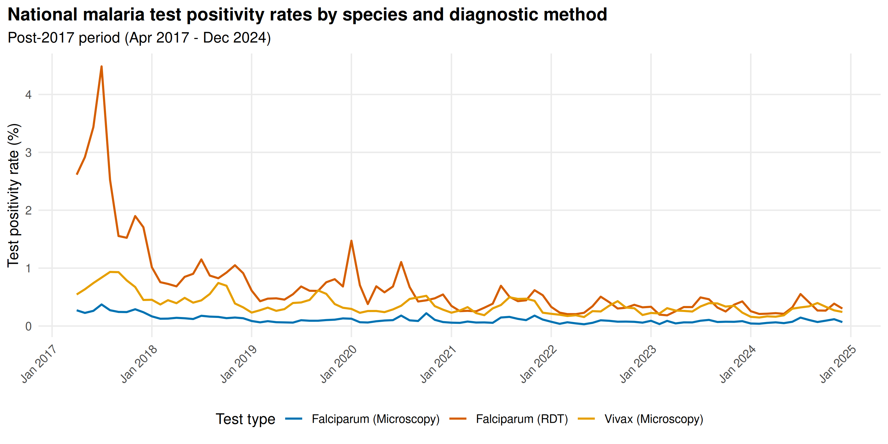
Both species peak July-October. Falciparum TPR exceeds Vivax nationally, reflecting P. falciparum dominance in the tribal belt. RDT Falciparum TPR runs lower than microscopy TPR.

State-level TPR for high-burden states

Top 5 states by total microscopy-confirmed cases (Vivax + Falciparum), with TPR trajectories:

# Total positive cases by state (microscopy only, for consistency)
state_burden <- vivax_micro |>
  bind_rows(falci_micro) |>
  group_by(state) |>
  summarise(total_positive = sum(value, na.rm = TRUE), .groups = "drop") |>
  arrange(desc(total_positive))

top5_states <- state_burden |>
  slice_head(n = 5) |>
  pull(state)

state_burden |>
  rename(State = state, `Total positive (microscopy)` = total_positive) |>
  datatable(
    options = list(pageLength = 10, scrollX = TRUE),
    rownames = FALSE,
    caption = "Total microscopy-confirmed malaria cases by state, Apr 2017 - Dec 2024"
  )

# Build state-level TPR for top 5
state_agg <- function(df, col_name) {
  df |>
    filter(state %in% top5_states) |>
    mutate(date = parse_monyear(monyear)) |>
    group_by(state, date) |>
    summarise(!!col_name := sum(value, na.rm = TRUE), .groups = "drop")
}

state_tpr <- state_agg(vivax_micro, "vivax_pos") |>
  inner_join(state_agg(falci_micro, "falci_pos"), by = c("state", "date")) |>
  inner_join(state_agg(smears_post, "smears"), by = c("state", "date")) |>
  mutate(
    tpr_vivax = vivax_pos / smears * 100,
    tpr_falci = falci_pos / smears * 100
  )

state_tpr_long <- state_tpr |>
  select(state, date, tpr_vivax, tpr_falci) |>
  pivot_longer(c(tpr_vivax, tpr_falci), names_to = "species", values_to = "tpr") |>
  mutate(species = ifelse(species == "tpr_vivax", "Vivax", "Falciparum"))

ggplot(state_tpr_long, aes(date, tpr, color = species)) +
  geom_line(linewidth = 0.7) +
  facet_wrap(~state, ncol = 1, scales = "free_y") +
  scale_color_manual(
    values = c("Vivax" = "#E69F00", "Falciparum" = "#0072B2"),
    name = "Species"
  ) +
  scale_x_date(date_labels = "%b %Y", date_breaks = "1 year") +
  labs(
    x = NULL,
    y = "Test positivity rate (%)",
    title = "Malaria TPR by species in top 5 high-burden states",
    subtitle = "Microscopy-confirmed, Apr 2017 - Dec 2024"
  ) +
  theme_minimal(base_size = 11) +
  theme(
    axis.text.x = element_text(angle = 45, hjust = 1),
    plot.title = element_text(face = "bold"),
    plot.title.position = "plot",
    panel.grid.minor = element_blank(),
    legend.position = "bottom",
    strip.text = element_text(face = "bold")
  )

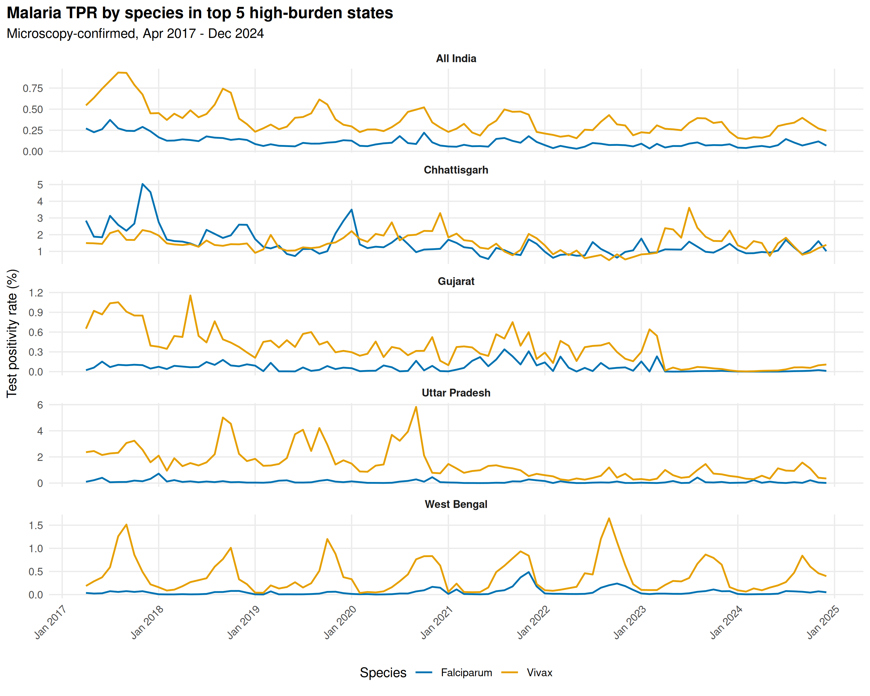
Forested tribal states are Falciparum-dominant; others show a more balanced species mix. The 2020 gap from COVID-19 lockdowns produces apparent TPR spikes: fewer tests performed, not more transmission.

3. Species composition shift

Fraction of microscopy-confirmed cases by species over time:

species_national <- agg(vivax_micro, "vivax") |>
  inner_join(agg(falci_micro, "falci"), by = "date") |>
  mutate(
    total = vivax + falci,
    frac_vivax = vivax / total,
    frac_falci = falci / total
  )

species_long <- species_national |>
  select(date, Vivax = frac_vivax, Falciparum = frac_falci) |>
  pivot_longer(-date, names_to = "species", values_to = "fraction")

ggplot(species_long, aes(date, fraction, fill = species)) +
  geom_area(alpha = 0.85) +
  scale_fill_manual(
    values = c("Vivax" = "#E69F00", "Falciparum" = "#0072B2"),
    name = "Species"
  ) +
  scale_x_date(date_labels = "%b %Y", date_breaks = "1 year") +
  scale_y_continuous(labels = scales::percent_format()) +
  labs(
    x = NULL,
    y = "Fraction of microscopy-confirmed cases",
    title = "Species composition of malaria in India (microscopy)",
    subtitle = "Stacked area chart, Apr 2017 - Dec 2024"
  ) +
  theme_minimal(base_size = 12) +
  theme(
    axis.text.x = element_text(angle = 45, hjust = 1),
    plot.title = element_text(face = "bold"),
    plot.title.position = "plot",
    panel.grid.minor = element_blank(),
    legend.position = "bottom"
  )

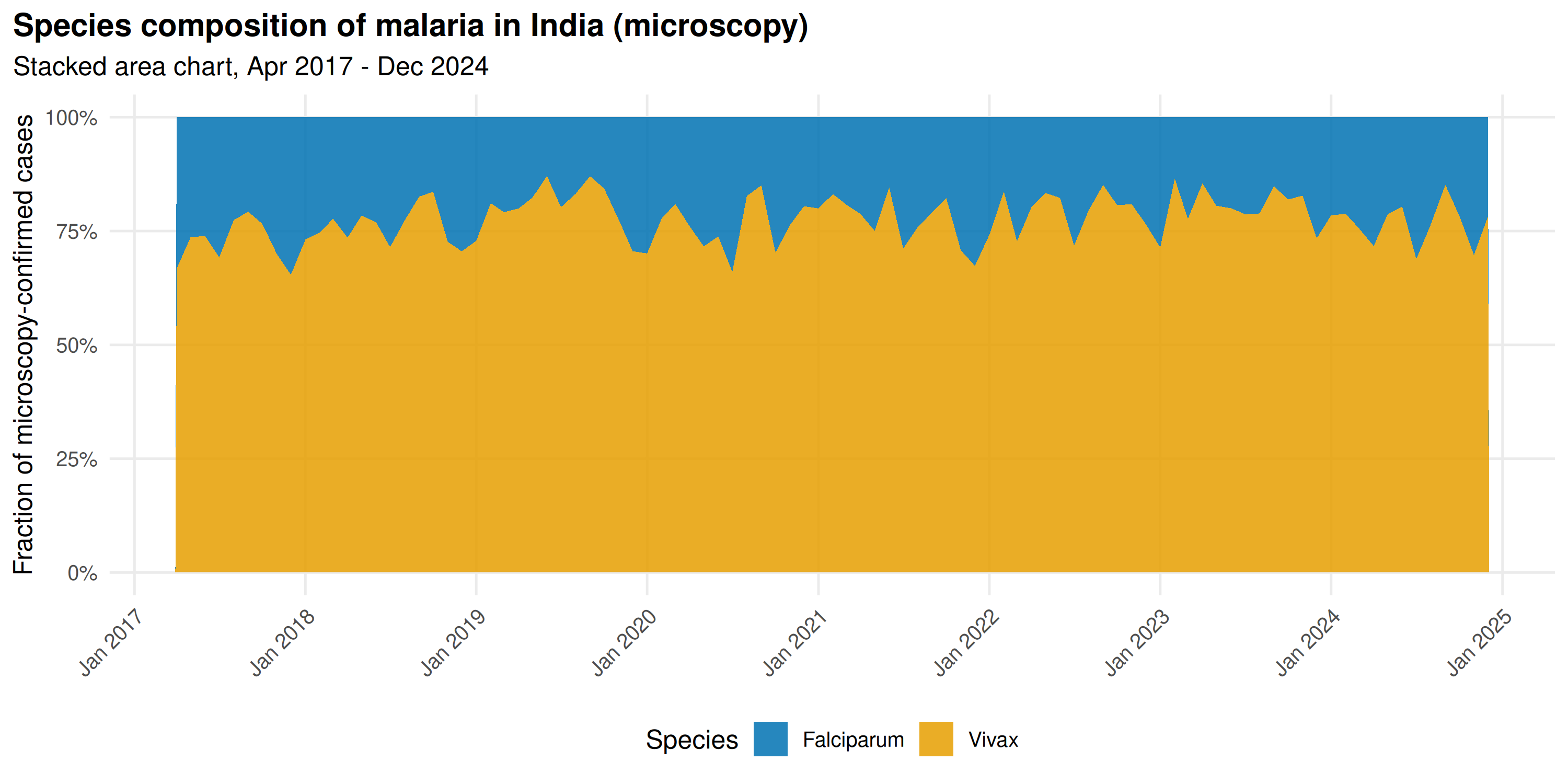
Falciparum dominates during monsoon peaks; Vivax holds a larger share in the off-season. P. vivax relapses from dormant liver-stage hypnozoites months after initial infection, sustaining year-round transmission. P. falciparum depends on active mosquito transmission during wet months.

Falciparum fraction by state

state_species <- vivax_micro |>
  mutate(date = parse_monyear(monyear)) |>
  group_by(state, date) |>
  summarise(vivax = sum(value, na.rm = TRUE), .groups = "drop") |>
  inner_join(
    falci_micro |>
      mutate(date = parse_monyear(monyear)) |>
      group_by(state, date) |>
      summarise(falci = sum(value, na.rm = TRUE), .groups = "drop"),
    by = c("state", "date")
  ) |>
  mutate(
    total = vivax + falci,
    falci_frac = ifelse(total > 0, falci / total, NA_real_)
  )

# Annual average Falciparum fraction by state
state_falci_annual <- state_species |>
  mutate(year = format(date, "%Y")) |>
  group_by(state, year) |>
  summarise(falci_frac = mean(falci_frac, na.rm = TRUE), .groups = "drop") |>
  mutate(year = as.Date(paste0(year, "-07-01")))

ggplot(state_falci_annual, aes(year, state, fill = falci_frac)) +
  geom_tile(color = "white", linewidth = 0.1) +
  scale_fill_viridis_c(
    option = "inferno",
    labels = scales::percent_format(),
    name = "Pf fraction"
  ) +
  scale_x_date(date_labels = "%Y", date_breaks = "1 year") +
  labs(
    x = NULL,
    y = NULL,
    title = "Falciparum fraction of malaria cases by state (annual average)",
    subtitle = "Darker = higher P. falciparum dominance"
  ) +
  theme_minimal(base_size = 11) +
  theme(
    axis.text.x = element_text(angle = 45, hjust = 1),
    plot.title = element_text(face = "bold"),
    plot.title.position = "plot",
    panel.grid = element_blank()
  )

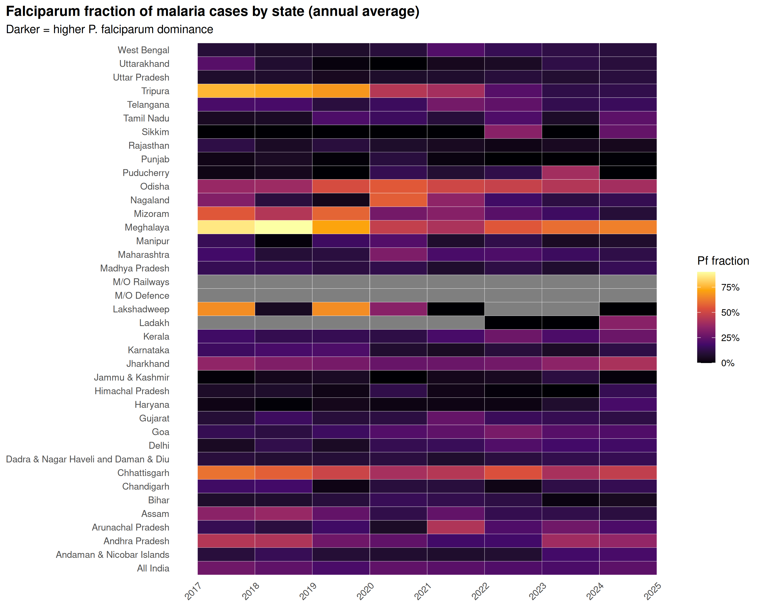
Northeastern states (Mizoram, Meghalaya, Tripura) and central-eastern tribal states (Odisha, Chhattisgarh, Jharkhand) are Falciparum-dominated. Northern and western states lean Vivax. Since P. falciparum causes severe malaria and most deaths, the Falciparum-dominant states need the most intensive case management.

4. Microscopy vs RDT comparison

Since April 2017, HMIS reports Falciparum positivity from microscopy and RDTs separately. RDTs detect the P. falciparum-specific HRP2 antigen and are designed for field use where microscopy is unavailable.

# State-month level TPR for both methods
micro_state <- falci_micro |>
  mutate(date = parse_monyear(monyear)) |>
  group_by(state, date) |>
  summarise(falci_micro_pos = sum(value, na.rm = TRUE), .groups = "drop")

rdt_pos_state <- falci_rdt |>
  mutate(date = parse_monyear(monyear)) |>
  group_by(state, date) |>
  summarise(falci_rdt_pos = sum(value, na.rm = TRUE), .groups = "drop")

smears_state <- smears_post |>
  mutate(date = parse_monyear(monyear)) |>
  group_by(state, date) |>
  summarise(smears_total = sum(value, na.rm = TRUE), .groups = "drop")

rdt_state <- rdt_conducted |>
  mutate(date = parse_monyear(monyear)) |>
  group_by(state, date) |>
  summarise(rdt_total = sum(value, na.rm = TRUE), .groups = "drop")

compare_tpr <- micro_state |>
  inner_join(rdt_pos_state, by = c("state", "date")) |>
  inner_join(smears_state, by = c("state", "date")) |>
  inner_join(rdt_state, by = c("state", "date")) |>
  mutate(
    micro_tpr = ifelse(smears_total > 0, falci_micro_pos / smears_total * 100, NA_real_),
    rdt_tpr   = ifelse(rdt_total > 0, falci_rdt_pos / rdt_total * 100, NA_real_)
  ) |>
  filter(
    !is.na(micro_tpr), !is.na(rdt_tpr),
    micro_tpr < 50, rdt_tpr < 50
  ) # exclude extreme outliers

ggplot(compare_tpr, aes(micro_tpr, rdt_tpr)) +
  geom_point(alpha = 0.3, size = 1.2, color = "#0072B2") +
  geom_abline(slope = 1, intercept = 0, linetype = "dashed", color = "grey50") +
  geom_smooth(
    method = "loess", se = TRUE, color = "#D55E00",
    fill = "#E69F00", alpha = 0.2, linewidth = 0.8
  ) +
  labs(
    x = "Microscopy Falciparum TPR (%)",
    y = "RDT Falciparum TPR (%)",
    title = "Microscopy vs RDT test positivity rates for P. falciparum",
    subtitle = "Each point = one state-month. Dashed line = perfect agreement."
  ) +
  theme_minimal(base_size = 12) +
  theme(
    plot.title = element_text(face = "bold"),
    plot.title.position = "plot",
    panel.grid.minor = element_blank()
  )

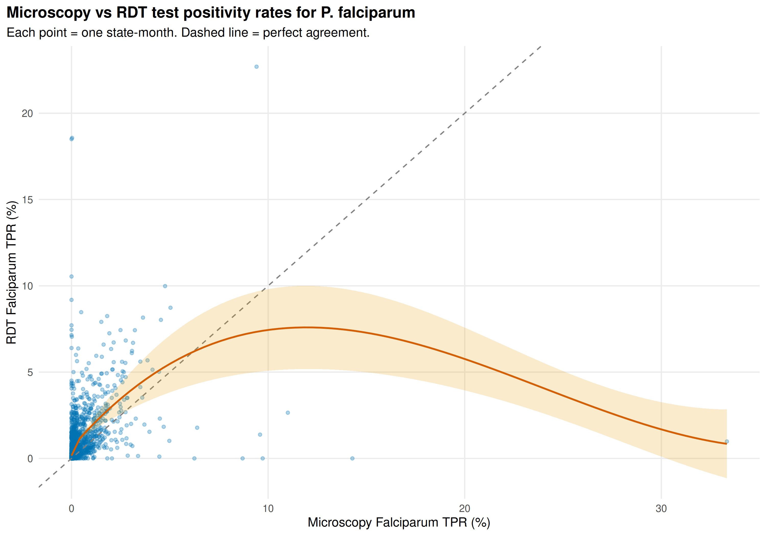
Most state-months cluster near zero. In higher-transmission settings, the LOESS curve bends below the diagonal: RDT TPR tends to be lower than microscopy TPR. RDTs can yield false negatives at low parasitaemia, and RDT denominators may be larger where RDTs are deployed for mass screening.

TPR ratio over time

ratio_national <- national_tpr |>
  mutate(
    ratio = ifelse(tpr_falci_micro > 0, tpr_falci_rdt / tpr_falci_micro, NA_real_)
  ) |>
  filter(!is.na(ratio))

ggplot(ratio_national, aes(date, ratio)) +
  geom_line(color = "#009E73", linewidth = 0.8) +
  geom_hline(yintercept = 1, linetype = "dashed", color = "grey50") +
  geom_smooth(
    method = "loess", span = 0.3, se = FALSE,
    color = "#D55E00", linewidth = 0.6
  ) +
  scale_x_date(date_labels = "%b %Y", date_breaks = "1 year") +
  labs(
    x = NULL,
    y = "RDT TPR / Microscopy TPR",
    title = "Ratio of RDT to microscopy Falciparum test positivity rates",
    subtitle = "Values < 1 indicate RDTs detect fewer positives per test than microscopy"
  ) +
  theme_minimal(base_size = 12) +
  theme(
    axis.text.x = element_text(angle = 45, hjust = 1),
    plot.title = element_text(face = "bold"),
    plot.title.position = "plot",
    panel.grid.minor = element_blank()
  )

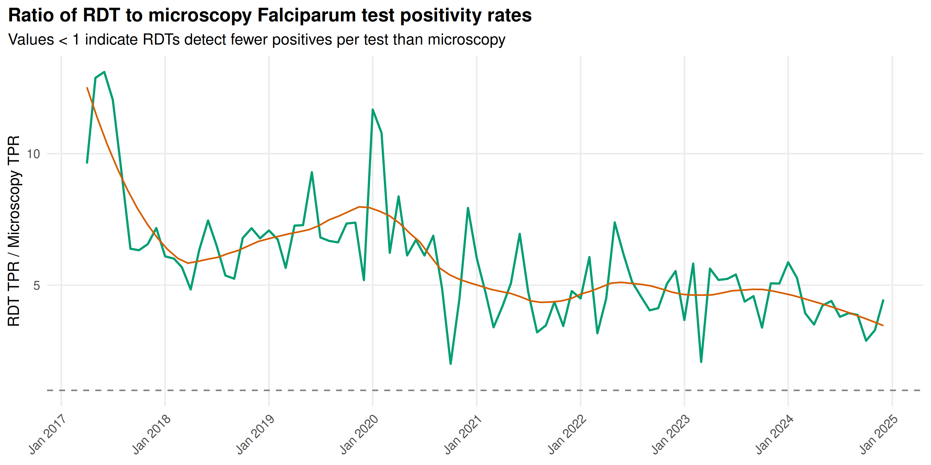
The ratio sits generally below 1.0: RDTs yield a systematically lower TPR than microscopy for Falciparum. As India shifts toward RDT-based screening in remote areas, apparent TPR will decline even if true transmission stays constant. Programmes should track method-specific TPR or adjust for diagnostic mix when assessing trends.

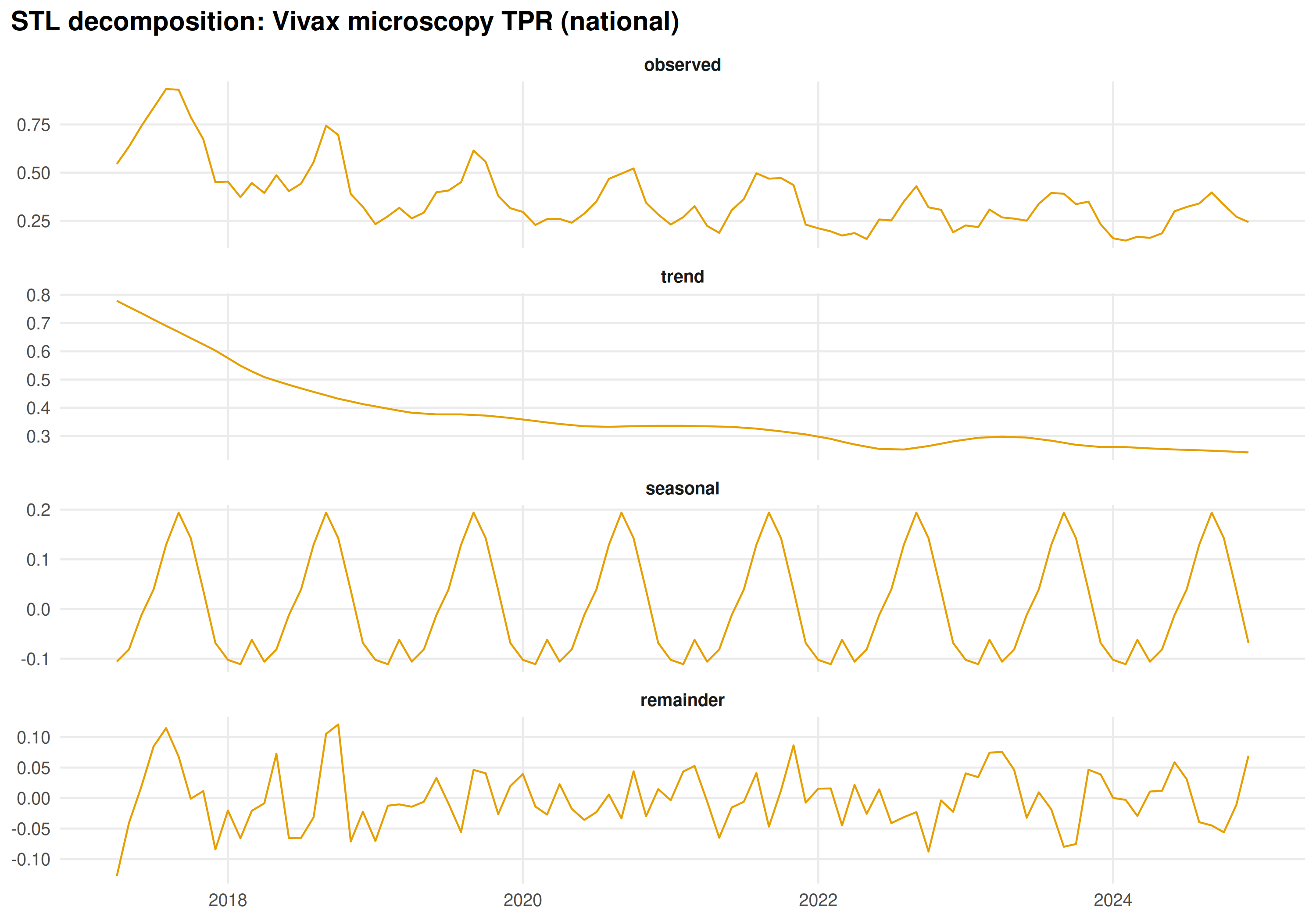
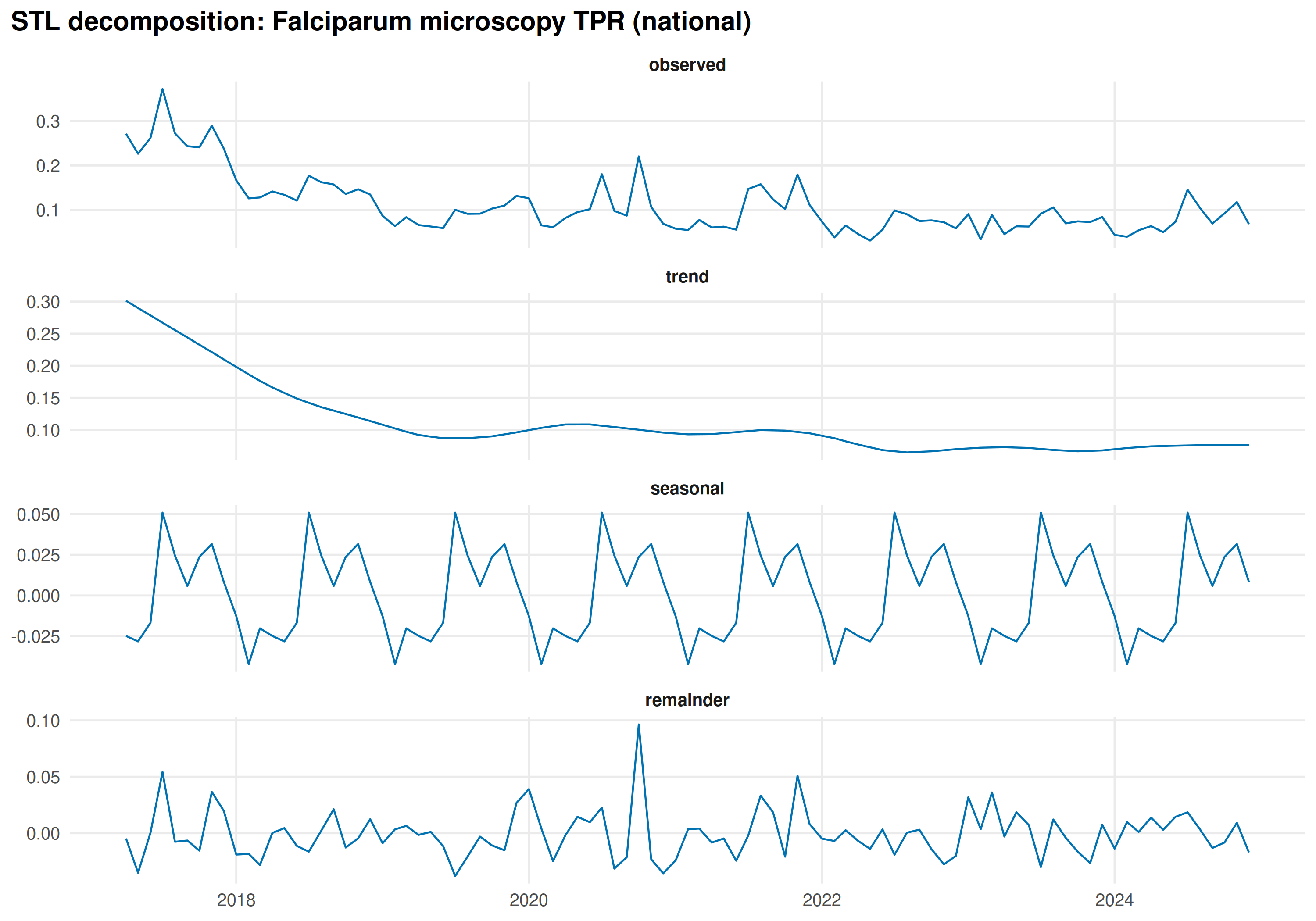
5. Seasonality of malaria

Both species show monsoon-driven seasonality. STL decomposition separates trend, seasonal, and residual components:

# National monthly TPR series for periodicity analysis
vivax_series <- national_tpr |>
  select(date, value = tpr_vivax_micro) |>
  mutate(monyear = format(date, "%b %Y")) |>
  filter(!is.na(value))

falci_series <- national_tpr |>
  select(date, value = tpr_falci_micro) |>
  mutate(monyear = format(date, "%b %Y")) |>
  filter(!is.na(value))

vivax_period <- detect_periodicity(vivax_series)
falci_period <- detect_periodicity(falci_series)

cat("Vivax TPR periodicity:\n")
#> Vivax TPR periodicity:
print(vivax_period)
#> Periodicity analysis (n = 93 observations)
#>   Detrended: TRUE
#>   Dominant period: 12 observations
#>   Spectral power concentration: 17 %
#>   ACF at dominant lag: 0.548 (threshold: 0.203 )
#> 
#> Top frequencies:
#>  period  power
#>    12.0 0.1073
#>    13.7 0.1062
#>    10.7 0.1053
#>    16.0 0.0588
#>     9.6 0.0537
cat("\nFalciparum TPR periodicity:\n")
#> 
#> Falciparum TPR periodicity:
print(falci_period)
#> Periodicity analysis (n = 93 observations)
#>   Detrended: TRUE
#>   Dominant period: 13.7 observations
#>   Spectral power concentration: 10.7 %
#>   ACF at dominant lag: 0.219 (threshold: 0.203 )
#> 
#> Top frequencies:
#>  period   power
#>    13.7 0.00739
#>    12.0 0.00689
#>    10.7 0.00631
#>    32.0 0.00586
#>    16.0 0.00476

Both species show strong 12-month periodicity. STL decomposition separates trend, seasonal, and residual components:

decomp_vivax <- decompose_series(vivax_series)

decomp_vivax_long <- decomp_vivax |>
  pivot_longer(
    cols = c(observed, trend, seasonal, remainder),
    names_to = "component", values_to = "val"
  ) |>
  mutate(component = factor(component,
    levels = c("observed", "trend", "seasonal", "remainder")
  ))

ggplot(decomp_vivax_long, aes(date, val)) +
  geom_line(color = "#E69F00", linewidth = 0.5) +
  facet_wrap(~component, ncol = 1, scales = "free_y") +
  labs(
    x = NULL, y = NULL,
    title = "STL decomposition: Vivax microscopy TPR (national)"
  ) +
  theme_minimal(base_size = 12) +
  theme(
    strip.text = element_text(face = "bold"),
    panel.grid.minor = element_blank(),
    plot.title = element_text(face = "bold"),
    plot.title.position = "plot"
  )

decomp_falci <- decompose_series(falci_series)

decomp_falci_long <- decomp_falci |>
  pivot_longer(
    cols = c(observed, trend, seasonal, remainder),
    names_to = "component", values_to = "val"
  ) |>
  mutate(component = factor(component,
    levels = c("observed", "trend", "seasonal", "remainder")
  ))

ggplot(decomp_falci_long, aes(date, val)) +
  geom_line(color = "#0072B2", linewidth = 0.5) +
  facet_wrap(~component, ncol = 1, scales = "free_y") +
  labs(
    x = NULL, y = NULL,
    title = "STL decomposition: Falciparum microscopy TPR (national)"
  ) +
  theme_minimal(base_size = 12) +
  theme(
    strip.text = element_text(face = "bold"),
    panel.grid.minor = element_blank(),
    plot.title = element_text(face = "bold"),
    plot.title.position = "plot"
  )

seasonal_compare <- data.frame(
  month = 1:12,
  Vivax = decomp_vivax |>
    mutate(month = as.numeric(format(date, "%m"))) |>
    group_by(month) |>
    summarise(s = mean(seasonal), .groups = "drop") |>
    pull(s),
  Falciparum = decomp_falci |>
    mutate(month = as.numeric(format(date, "%m"))) |>
    group_by(month) |>
    summarise(s = mean(seasonal), .groups = "drop") |>
    pull(s)
) |>
  pivot_longer(-month, names_to = "species", values_to = "seasonal")

ggplot(seasonal_compare, aes(month, seasonal, color = species)) +
  geom_line(linewidth = 1) +
  geom_point(size = 2) +
  geom_hline(yintercept = 0, linetype = "dashed", color = "grey50") +
  scale_x_continuous(
    breaks = 1:12,
    labels = month.abb
  ) +
  scale_color_manual(
    values = c("Vivax" = "#E69F00", "Falciparum" = "#0072B2"),
    name = "Species"
  ) +
  labs(
    x = NULL,
    y = "Seasonal component (TPR deviation)",
    title = "Average seasonal profile: Vivax vs Falciparum TPR",
    subtitle = "Extracted from STL decomposition of national monthly TPR"
  ) +
  theme_minimal(base_size = 12) +
  theme(
    plot.title = element_text(face = "bold"),
    plot.title.position = "plot",
    panel.grid.minor = element_blank(),
    legend.position = "bottom"
  )

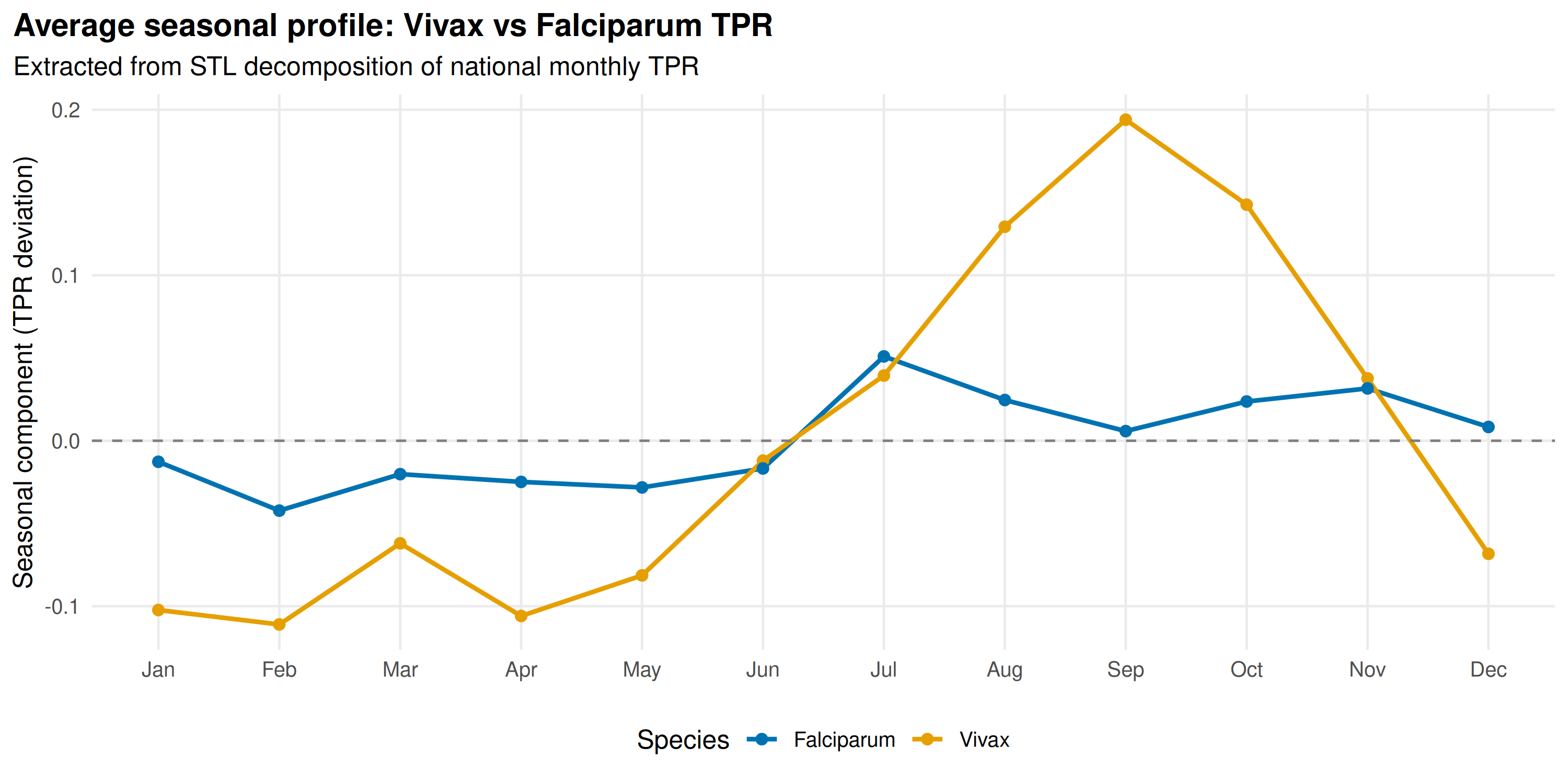
P. falciparum has a sharper peak concentrated in wet-month transmission. P. vivax spans a broader window, sustained by hypnozoite relapses after the monsoon ends.

6. State-level summary table

Summary table: mean TPRs, dominant species, and peak transmission month by state.

# State-month level TPR for all three metrics
state_detail <- micro_state |>
  inner_join(rdt_pos_state, by = c("state", "date")) |>
  inner_join(smears_state, by = c("state", "date")) |>
  inner_join(rdt_state, by = c("state", "date")) |>
  inner_join(
    vivax_micro |>
      mutate(date = parse_monyear(monyear)) |>
      group_by(state, date) |>
      summarise(vivax_pos = sum(value, na.rm = TRUE), .groups = "drop"),
    by = c("state", "date")
  ) |>
  mutate(
    tpr_vivax_micro  = ifelse(smears_total > 0, vivax_pos / smears_total * 100, NA_real_),
    tpr_falci_micro  = ifelse(smears_total > 0, falci_micro_pos / smears_total * 100, NA_real_),
    tpr_falci_rdt    = ifelse(rdt_total > 0, falci_rdt_pos / rdt_total * 100, NA_real_),
    total_pos        = vivax_pos + falci_micro_pos,
    month_num        = as.numeric(format(date, "%m"))
  )

# Summarise by state
state_summary <- state_detail |>
  group_by(state) |>
  summarise(
    mean_tpr_vivax = round(mean(tpr_vivax_micro, na.rm = TRUE), 3),
    mean_tpr_falci = round(mean(tpr_falci_micro, na.rm = TRUE), 3),
    mean_tpr_falci_rdt = round(mean(tpr_falci_rdt, na.rm = TRUE), 3),
    total_vivax = sum(vivax_pos, na.rm = TRUE),
    total_falci = sum(falci_micro_pos, na.rm = TRUE),
    .groups = "drop"
  ) |>
  mutate(
    dominant_species = ifelse(total_falci > total_vivax, "Pf", "Pv")
  )

# Peak month (month with highest average total positives)
peak_months <- state_detail |>
  group_by(state, month_num) |>
  summarise(avg_pos = mean(total_pos, na.rm = TRUE), .groups = "drop") |>
  group_by(state) |>
  slice_max(avg_pos, n = 1, with_ties = FALSE) |>
  ungroup() |>
  mutate(peak_month = month.abb[month_num]) |>
  select(state, peak_month)

state_summary <- state_summary |>
  left_join(peak_months, by = "state") |>
  select(
    State = state,
    `Mean TPR Vivax (%)` = mean_tpr_vivax,
    `Mean TPR Falci micro (%)` = mean_tpr_falci,
    `Mean TPR Falci RDT (%)` = mean_tpr_falci_rdt,
    `Dominant species` = dominant_species,
    `Peak month` = peak_month
  ) |>
  arrange(desc(`Mean TPR Falci micro (%)`))

state_summary |>
  datatable(
    filter = "top",
    options = list(pageLength = 15, scrollX = TRUE),
    rownames = FALSE,
    caption = "State-level malaria summary, Apr 2017 - Dec 2024 (microscopy TPR = positives / blood smears)"
  )

States with high Falciparum TPR and late-monsoon peaks need intensive case management and vector control during those months. Vivax-dominant states need a different approach: radical cure with primaquine to clear hypnozoites and prevent relapses.