Maternal deaths

#  OLD SERIES: Apr 2008–Mar 2017
mat_abortion_old <- get_hmis(
  "Number of cases of Maternal deaths (age 15 - 49 years) with the probable cause being Abortion",
  sector = "Total", to = "Mar 2017"
) |> add_calendar_vars() |> mutate(cause = "Abortion", series = "old")

# Bleeding = PPH proxy in old series. Ends Mar 2017 — NEVER resumed.
mat_pph_old <- get_hmis(
  "Number of cases of Maternal deaths (age 15 - 49 years) with the probable cause being Bleeding",
  sector = "Total", to = "Mar 2017"
) |> add_calendar_vars() |> mutate(cause = "Haemorrhage (PPH)", series = "old")

mat_fever_old <- get_hmis(
  "Number of cases of Maternal deaths (age 15 - 49 years) with the probable cause being High Fever",
  sector = "Total", to = "Mar 2017"
) |> add_calendar_vars() |> mutate(cause = "High Fever / Infection", series = "old")

mat_obstructed_old <- get_hmis(
  "Number of cases of Maternal deaths (age 15 - 49 years) with the probable cause being Obstructed",
  match = "fixed", sector = "Total", to = "Mar 2017"
) |> add_calendar_vars() |> mutate(cause = "Obstructed Labour", series = "old")

mat_other_old <- get_hmis(
  "Number of cases of Maternal deaths (age 15 - 49 years) with the probable cause being other cause",
  match = "fixed", sector = "Total", to = "Mar 2017"
) |> add_calendar_vars() |> mutate(cause = "Other", series = "old")

mat_hypert_old <- get_hmis(
  "Number of cases of Maternal deaths (age 15 - 49 years) with the probable cause being Severe hype",
  match = "fixed", sector = "Total", to = "Mar 2017"
) |> add_calendar_vars() |> mutate(cause = "Hypertension/Eclampsia", series = "old")

#  NEW SERIES: Apr 2017–Apr 2025
mat_abortion_new <- get_hmis(
  "Number of Maternal Deaths due to Abortion",
  sector = "Total", from = "Apr 2017"
) |> add_calendar_vars() |> mutate(cause = "Abortion", series = "new")

# High fever ends Mar 2023 — replaced by Infection/Sepsis indicator from Apr 2023
mat_fever_new <- get_hmis(
  "Number of Maternal Deaths due to High fever",
  sector = "Total", from = "Apr 2017", to = "Mar 2023"
) |> add_calendar_vars() |> mutate(cause = "High Fever / Infection", series = "new")

# Infection/Sepsis: Apr 2023 onwards — continuation of High Fever concept
mat_infection_new <- get_hmis(
  "Number of Maternal Deaths due to Pregnancy related infection and sepsis, Fever",
  sector = "Total", from = "Apr 2023"
) |> add_calendar_vars() |> mutate(cause = "High Fever / Infection", series = "new")

mat_obstructed_new <- get_hmis(
  "Number of Maternal Deaths due to Obstructed/prolonged labour",
  sector = "Total", from = "Apr 2017"
) |> add_calendar_vars() |> mutate(cause = "Obstructed Labour", series = "new")

mat_other_new <- get_hmis(
  "Number of Maternal Deaths due to Other Causes (including causes not known)",
  sector = "Total", from = "Apr 2017"
) |> add_calendar_vars() |> mutate(cause = "Other", series = "new")

# filter by exact canonical_name to avoid double-counting
# with the Apr 2023 detailed Hypertension indicator
mat_hypert_new <- get_hmis(
  "Number of Maternal Deaths due to Severe hypertension/fits",
  sector = "Total", from = "Apr 2017"
) |>
  dplyr::filter(
    canonical_name == "Number of Maternal Deaths due to Severe hypertension/fits"
  ) |>
  add_calendar_vars() |>
  mutate(cause = "Hypertension/Eclampsia", series = "new")

#  Combine all causes
# Note: High Fever (old/new) + Infection/Sepsis (Apr 2023) combined under
# "High Fever / Infection" as they represent the same broad clinical concept
all_causes_mmr <- bind_rows(
  mat_abortion_old,   mat_pph_old,         mat_fever_old,
  mat_obstructed_old, mat_other_old,        mat_hypert_old,
  mat_abortion_new,   mat_fever_new,        mat_infection_new,
  mat_obstructed_new, mat_other_new,        mat_hypert_new
) |>
  filter(!state %in% exclude_states) |>
  mutate(cause = factor(cause, levels = c(
    "Hypertension/Eclampsia", "Haemorrhage (PPH)",
    "High Fever / Infection", "Obstructed Labour",
    "Abortion", "Other"
  )))

Live births

# Live births 
births_old <- get_hmis(
  "Total number of male and female live births",
  sector = "Total", to = "Mar 2017"
) |> add_calendar_vars()

births_new <- bind_rows(
  get_hmis("Number of male live births",   sector = "Total", from = "Apr 2017"),
  get_hmis("Number of female live births", sector = "Total", from = "Apr 2017")
) |> add_calendar_vars()

b_collapsed <- bind_rows(births_old, births_new) |>
  filter(!state %in% exclude_states) |>
  group_by(state, monyear, cal_year, month, month_num) |>
  summarise(births = sum(as.numeric(value), na.rm = TRUE), .groups = "drop")

Calculate MMR

# State × cause annual MMR (new series only — consistent)
mmr_state_annual <- mmr_data |>
  filter(
    cal_year >= 2018, cal_year <= 2024,
    series == "new",
    !state %in% exclude_states,
    state != "All India"
  ) |>
  group_by(state, cal_year, cause) |>
  summarise(
    total_deaths = sum(deaths, na.rm = TRUE),
    total_births = sum(births, na.rm = TRUE),
    mmr          = (total_deaths / total_births) * 100000,
    .groups      = "drop"
  )

This vignette examines how maternal mortality in India has changed since 2008, how it varies across causes and states, and whether it shows seasonal patterns.

Critical data gap. Haemorrhage (PPH) was discontinued from HMIS after March 2017, despite being the leading cause of maternal death globally. All post-2017 analyses in this vignette are therefore systematically incomplete. Where this affects interpretation it is flagged explicitly.

Indicator coverage

tibble::tribble(
  ~Cause,                    ~`Old series`,      ~`New series`,        ~Note,
  "Abortion",                "Apr 2008–Mar 2017", "Apr 2017–Apr 2025",  "Continuous",
  "Haemorrhage (PPH)",       "Apr 2008–Mar 2017", "DROPPED",            "Missing post-2017",
  "High Fever / Infection",  "Apr 2008–Mar 2017", "Apr 2017–Mar 2023",  "Renamed Apr 2023",
  "Obstructed Labour",       "Apr 2008–Mar 2017", "Apr 2017–Apr 2025",  "Continuous",
  "Hypertension/Eclampsia",  "Apr 2008–Mar 2017", "Apr 2017–Apr 2025",  "Continuous",
  "Other",                   "Apr 2008–Mar 2017", "Apr 2017–Apr 2025",  "Continuous",
  "Infection/Sepsis",        "–",                 "Apr 2023–Apr 2025",  "New — replaces High Fever",
  "Detailed Hypertension",   "–",                 "Apr 2023–Apr 2025",  "New — more specific"
) |>
  gt() |>
  tab_header(
    title    = md("**HMIS Maternal Death Indicator Coverage**"),
    subtitle = md("All India | Apr 2008–Apr 2025")
  ) |>
  tab_style(
    style     = cell_text(color = "grey39", weight = "bold"),
    locations = cells_body(
      columns = `New series`,
      rows    = `New series` == "DROPPED"
    )
  ) |>
  tab_style(
    style     = cell_text(color = "tan3"),
    locations = cells_body(
      columns = Note,
      rows    = Note != "Continuous"
    )
  ) |>
  tab_footnote(
    footnote  = "Haemorrhage (PPH) is the leading cause of maternal death globally (WHO). Its absence from post-2017 HMIS data means all post-2017 MMR estimates are underestimates.",
    locations = cells_body(columns = Cause, rows = Cause == "Haemorrhage (PPH)")
  ) |>
  opt_stylize(style = 1)

Cause	Old series	New series	Note
HMIS Maternal Death Indicator Coverage
All India \| Apr 2008–Apr 2025
Abortion	Apr 2008–Mar 2017	Apr 2017–Apr 2025	Continuous
Haemorrhage (PPH)¹	Apr 2008–Mar 2017	DROPPED	Missing post-2017
High Fever / Infection	Apr 2008–Mar 2017	Apr 2017–Mar 2023	Renamed Apr 2023
Obstructed Labour	Apr 2008–Mar 2017	Apr 2017–Apr 2025	Continuous
Hypertension/Eclampsia	Apr 2008–Mar 2017	Apr 2017–Apr 2025	Continuous
Other	Apr 2008–Mar 2017	Apr 2017–Apr 2025	Continuous
Infection/Sepsis	–	Apr 2023–Apr 2025	New — replaces High Fever
Detailed Hypertension	–	Apr 2023–Apr 2025	New — more specific
¹ Haemorrhage (PPH) is the leading cause of maternal death globally (WHO). Its absence from post-2017 HMIS data means all post-2017 MMR estimates are underestimates.

National MMR trend by cause

ggplot(
  mmr_national_annual,
  aes(x = cal_year, y = mmr, color = cause, group = cause)
) +
  geom_vline(xintercept = 2017, linetype = "dotted",
             color = "grey50", linewidth = 0.7) +
  annotate("text", x = 2017.2, y = Inf, vjust = 1.5,
           hjust = 0, size = 2.8, color = "grey40",
           label = "Apr 2017\nindicator rename") +
  # PPH ends — mark it
  annotate("segment",
           x = 2017, xend = 2017,
           y = -Inf, yend = Inf,
           color = "black", linewidth = 0.4, linetype = "dashed") +
  geom_line(linewidth = 1, na.rm = TRUE) +
  scale_color_manual(values = cause_colours, name = NULL) +
  scale_x_continuous(breaks = seq(2008, 2024, 2)) +
  scale_y_continuous(labels = number_format(accuracy = 0.1)) +
  labs(
    title    = "Maternal Mortality Ratio by cause — All India (2008–2024)",
    subtitle = "MMR = maternal deaths per 100,000 live births | Facility-reported only",
    caption  = paste0(
      "Haemorrhage (PPH) ends Mar 2017 — data gap, not health gain\n",
      "High Fever series ends Mar 2023, replaced by Infection/Sepsis from Apr 2023\n",
      "Source: HMIS via hmisindia"
    ),
    x = NULL, y = "MMR (per 100,000 live births)"
  ) +
  theme_hmis() +
    labs_hmis()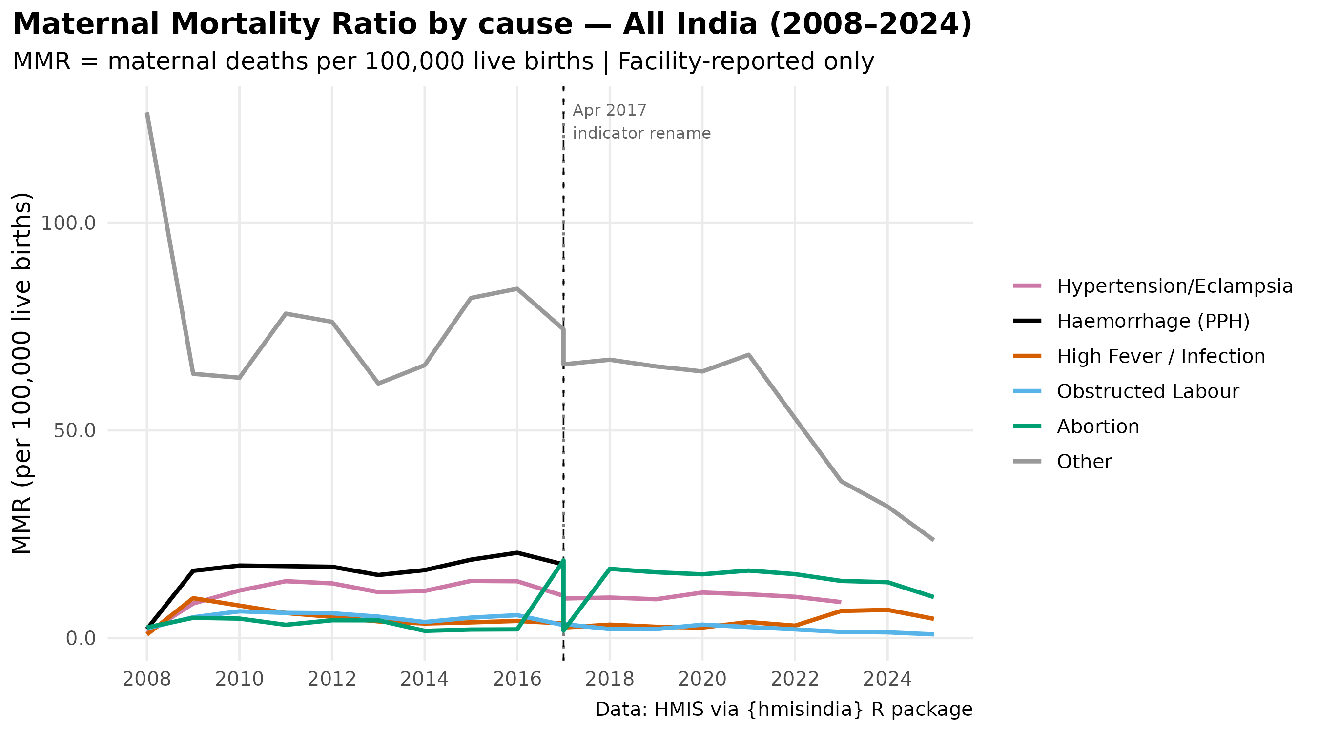

State-level MMR distribution

mmr_state_annual |>
  filter(cause != "Other") |>
  ggplot(aes(
    x = reorder(state, mmr, FUN = median, na.rm = TRUE),
    y = mmr
  )) +
  geom_boxplot(fill = "snow", alpha = 0.7,
               outlier.size = 0.8, outlier.alpha = 0.5) +
  coord_flip() +
  facet_wrap(~cause, scales = "free_x", nrow = 1) +
  labs(
    title    = "MMR distribution by state and cause (2018–2024)",
    subtitle = "New indicator series only | States ordered by median MMR",
    caption  = "Source: HMIS via hmisindia | Facility-reported deaths only",
    x = NULL, y = "MMR (per 100,000 live births)"
  ) +
  theme_hmis() +
  theme(
    axis.text.y  = element_text(size = 7),
    strip.text   = element_text(face = "bold", size = 8),
    axis.text.x  = element_text(size = 7)
  ) +
    labs_hmis()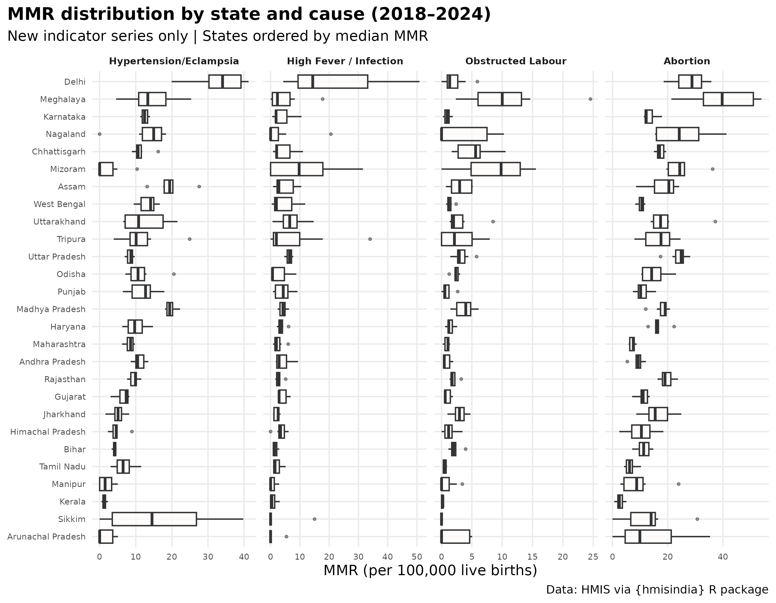

State × year heatmap — which states improved?

# Total MMR per state per year (all causes summed, new series)
mmr_total_state <- mmr_state_annual |>
  group_by(state, cal_year) |>
  summarise(
    total_deaths = sum(total_deaths, na.rm = TRUE),
    total_births = sum(total_births, na.rm = TRUE),
    mmr          = (total_deaths / total_births) * 100000,
    .groups      = "drop"
  )

# Order states by 2018 MMR
state_order_2018 <- mmr_total_state |>
  filter(cal_year == 2018) |>
  arrange(desc(mmr)) |>
  pull(state)

mmr_total_state |>
  mutate(state = factor(state, levels = state_order_2018)) |>
  ggplot(aes(x = factor(cal_year), y = state, fill = mmr)) +
  geom_tile(color = "white", linewidth = 0.3) +
  scale_fill_distiller(
    palette   = "YlOrRd",
    direction = 1,
    name      = "MMR\n(per 100k\nlive births)",
    na.value  = "grey80"
  ) +
  labs(
    title    = "Total MMR by state and year (2018–2024)",
    subtitle = "States ordered by 2018 MMR | Lighter = improvement | New series only",
    caption  = paste0(
      "Haemorrhage (PPH) NOT included — discontinued post-2017\n",
      "MMR values are underestimates | Source: HMIS via hmisindia"
    ),
    x = NULL, y = NULL
  ) +
  theme_hmis() +
  theme(
    panel.grid      = element_blank(),
    axis.text.y     = element_text(size = 8, face = "bold"),
    legend.position = "right"
  ) +
    labs_hmis()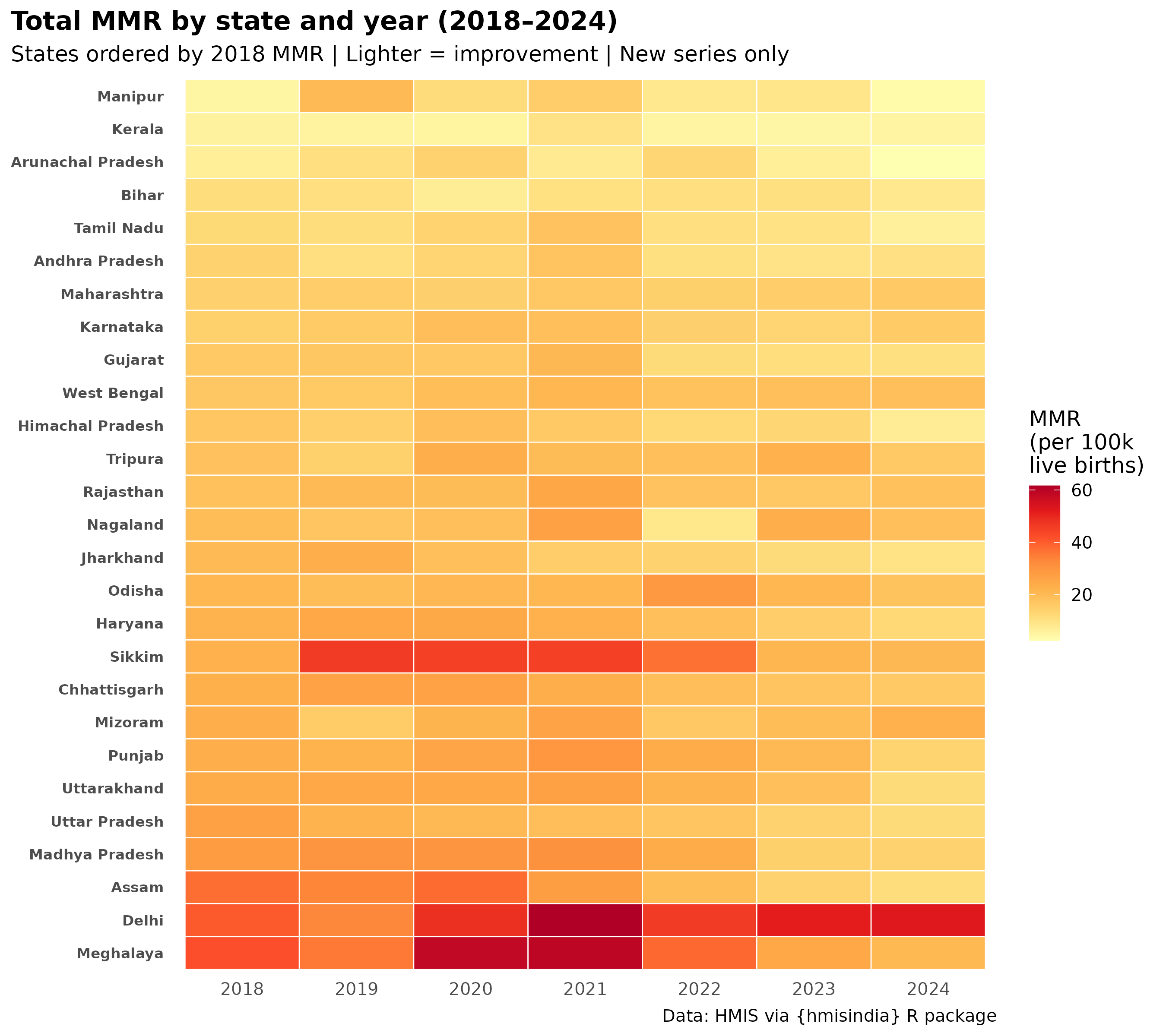

Cause composition by state

mmr_state_cause_avg <- mmr_state_annual |>
  filter(cause != "Other") |>
  group_by(state, cause) |>
  summarise(avg_mmr = mean(mmr, na.rm = TRUE), .groups = "drop") |>
  group_by(state) |>
  mutate(
    total_mmr = sum(avg_mmr, na.rm = TRUE),
    pct       = avg_mmr / total_mmr * 100
  ) |>
  ungroup()

state_order_hypert <- mmr_state_cause_avg |>
  filter(cause == "Hypertension/Eclampsia") |>
  arrange(desc(pct)) |>
  pull(state)

mmr_state_cause_avg |>
  mutate(state = factor(state, levels = state_order_hypert)) |>
  ggplot(aes(x = pct, y = state, fill = cause)) +
  geom_bar(stat = "identity", position = "stack") +
  scale_fill_manual(values = cause_colours, name = NULL) +
  scale_x_continuous(labels = percent_format(scale = 1)) +
  labs(
    title    = "Cause composition of MMR by state (2018–2024)",
    subtitle = "States ordered by Hypertension share | Other excluded for clarity",
    caption  = paste0(
      "Haemorrhage (PPH) not shown — data unavailable post-2017\n",
      "Source: HMIS via hmisindia"
    ),
    x = "% of total MMR", y = NULL
  ) +
  theme_hmis() +
  theme(axis.text.y = element_text(size = 8, face = "bold")) +
    labs_hmis()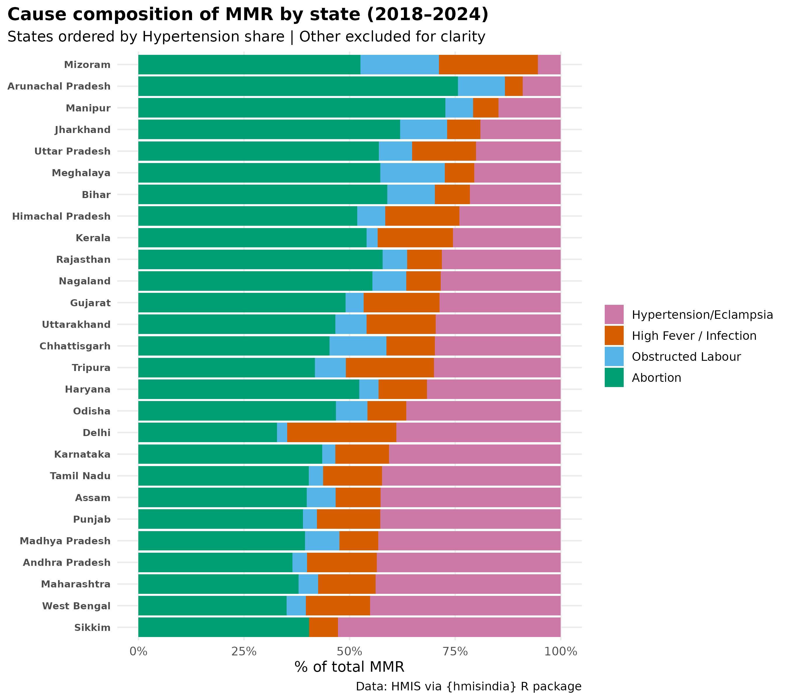

Seasonality

The hmis_seasonality dataset contains pre-computed seasonal statistics. Nine maternal indicators are available. Review indicators (MDR, FBMDR, CBMDR) are excluded — they count reviews, not deaths.

# Indicators available in hmis_seasonality for maternal deaths
maternal_seasonality_indicators <- c(
  # New series
  "Number of Maternal Deaths due to Severe hypertension/fits",
  "Number of Maternal Deaths due to Abortion",
  "Number of Maternal Deaths due to Other Causes (including causes not known)",
  "Number of Maternal Deaths due to High fever",
  # Old series
  "Number of cases of Maternal deaths (age 15 - 49 years) with the probable cause being Bleeding",
  "Number of cases of Maternal deaths (age 15 - 49 years) with the probable cause being Abortion",
  "Number of cases of Maternal deaths (age 15 - 49 years) with the probable cause being Obstructed",
  "Number of cases of Maternal deaths (age 15 - 49 years) with the probable cause being Severe hype",
  "Number of cases of Maternal deaths (age 15 - 49 years) with the probable cause being High Fever"
)

mat_seasonality <- hmis_seasonality |>
  dplyr::filter(canonical_name %in% maternal_seasonality_indicators) |>
  dplyr::mutate(
    series = dplyr::if_else(
      grepl("cases of Maternal", canonical_name),
      "Old (2008–2017)", "New (2017–2025)"
    ),
    cause_short = dplyr::case_when(
      grepl("hypertension|fits|Severe hype", canonical_name,
            ignore.case = TRUE)              ~ "Hypertension/Eclampsia",
      grepl("Bleeding|bleeding",   canonical_name) ~ "Haemorrhage (PPH)",
      grepl("Abortion|abortion",   canonical_name) ~ "Abortion",
      grepl("Obstructed|prolonged|Obstructed",
            canonical_name)                        ~ "Obstructed Labour",
      grepl("fever|Fever|infection",
            canonical_name,
            ignore.case = TRUE)                    ~ "High Fever / Infection",
      grepl("Other Causes|other cause",
            canonical_name)                        ~ "Other",
      TRUE ~ canonical_name
    )
  ) |>
  dplyr::select(series, cause_short, peak_month,
                seasonal_strength, amplitude_pct, seasonality) |>
  dplyr::arrange(series, dplyr::desc(seasonal_strength))

mat_seasonality |>
  gt() |>
  tab_header(
    title    = md("**Seasonality of maternal deaths by cause**"),
    subtitle = md("Pre-computed from `hmis_seasonality` | All India")
  ) |>
  cols_label(
    series           = "Series",
    cause_short      = "Cause",
    peak_month       = "Peak month",
    seasonal_strength = "Seasonal strength",
    amplitude_pct    = "Amplitude (%)",
    seasonality      = "Classification"
  ) |>
  fmt_number(columns = c(seasonal_strength, amplitude_pct), decimals = 2) |>
  data_color(columns = seasonal_strength, palette = "Oranges") |>
  tab_footnote(
    footnote  = "Seasonal strength: 0 = flat, 1 = perfectly seasonal",
    locations = cells_column_labels(columns = seasonal_strength)
  ) |>
  tab_source_note(
    "Obstructed Labour not in hmis_seasonality — compute directly if needed"
  ) |>
  opt_stylize(style = 1)

Series	Cause	Peak month	Seasonal strength¹	Amplitude (%)	Classification
Seasonality of maternal deaths by cause
Pre-computed from `hmis_seasonality` \| All India
New (2017–2025)	Hypertension/Eclampsia	Sep	0.77	49.26	strong
New (2017–2025)	Abortion	Sep	0.70	55.77	strong
New (2017–2025)	Other	Sep	0.41	49.32	moderate
New (2017–2025)	High Fever / Infection	Sep	0.40	89.05	moderate
Old (2008–2017)	Haemorrhage (PPH)	Sep	0.52	40.54	moderate
Old (2008–2017)	Haemorrhage (PPH)	Sep	0.50	40.71	moderate
¹ Seasonal strength: 0 = flat, 1 = perfectly seasonal
Obstructed Labour not in hmis_seasonality — compute directly if needed

mat_seasonality |>
  ggplot(aes(
    x    = reorder(cause_short, seasonal_strength),
    y    = seasonal_strength,
    fill = peak_month
  )) +
  geom_col(width = 0.7, alpha = 0.9) +
  geom_text(
    aes(label = paste0(peak_month, " (", round(seasonal_strength, 2), ")")),
    hjust = -0.1, size = 3
  ) +
  coord_flip() +
  facet_wrap(~series, scales = "free_y") +
  scale_fill_manual(
    values = c(
      "Sep" = "#D55E00", "Aug" = "#E69F00",
      "Jun" = "#56B4E9", "Dec" = "#0072B2",
      "Jul" = "#009E73"
    ),
    name = "Peak month",
    na.value = "grey70"
  ) +
  scale_y_continuous(
    limits = c(0, 1),
    expand = expansion(mult = c(0, 0.3))
  ) +
  labs(
    title    = "Seasonal strength of maternal deaths by cause",
    subtitle = "Label = peak month | Higher = stronger seasonality",
    caption  = paste0(
      "Obstructed Labour not available in hmis_seasonality\n",
      "Source: hmis_seasonality dataset | hmisindia package"
    ),
    x = NULL, y = "Seasonal strength (0–1)"
  ) +
  theme_hmis() +
    labs_hmis()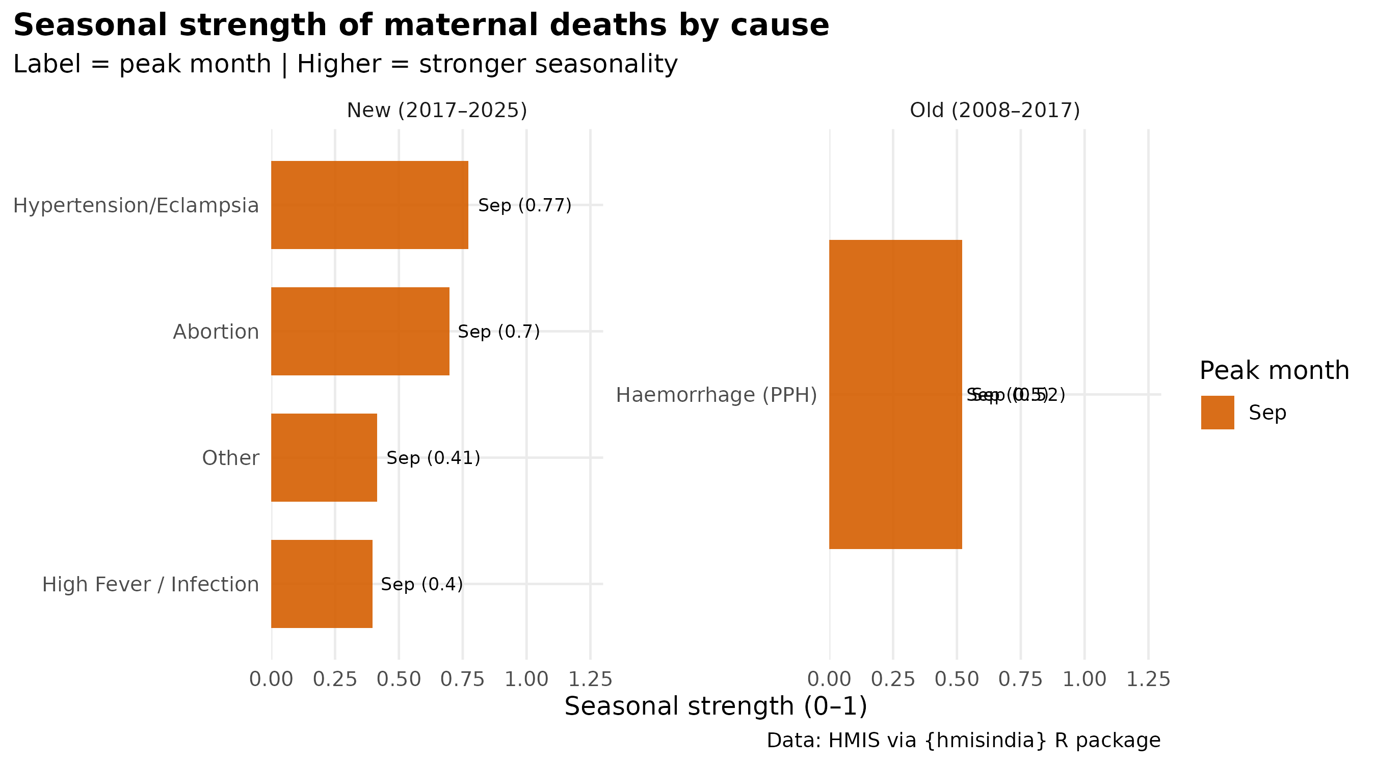

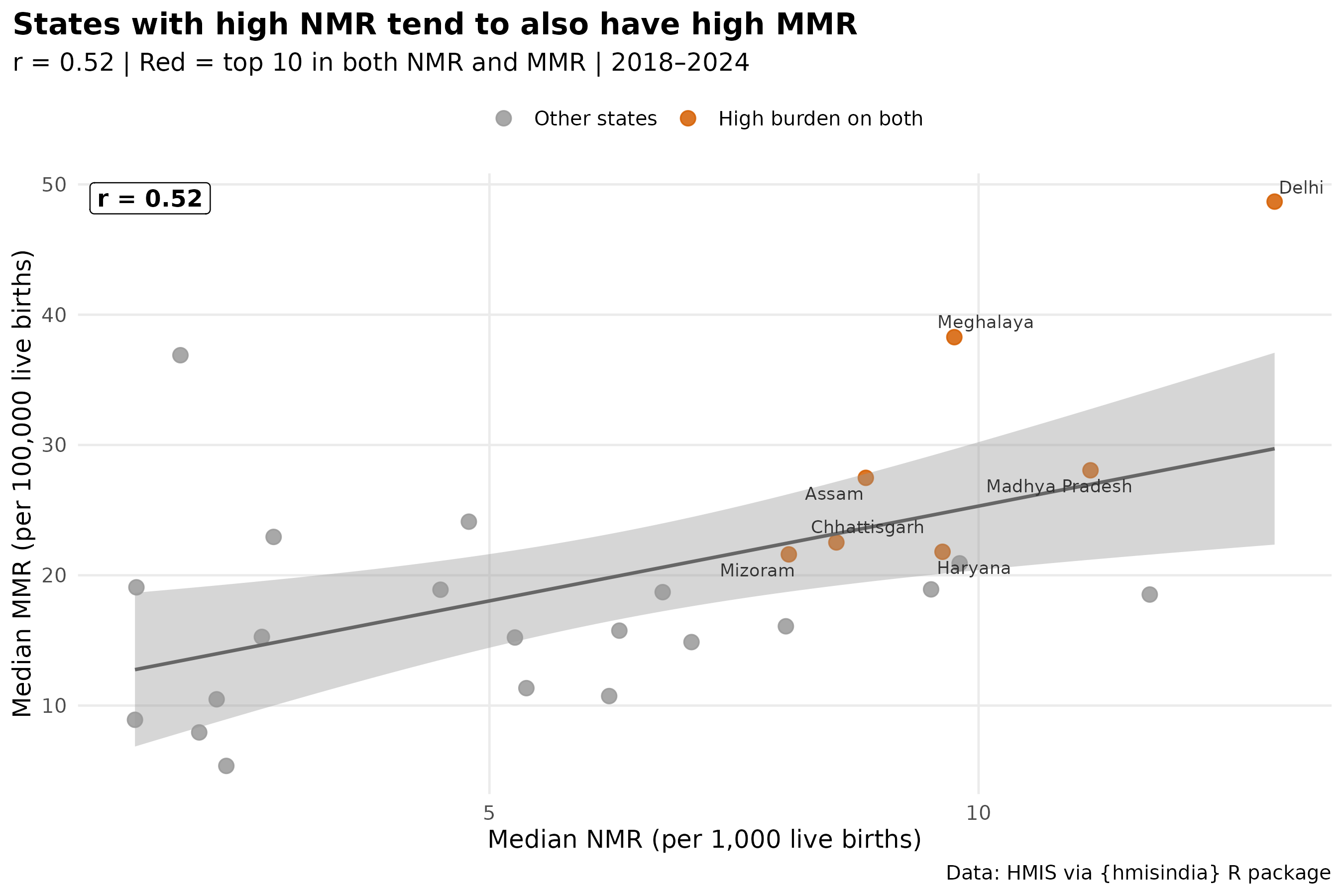
7. Are high-MMR states also high-NMR states?

# Requires nmr_state_annual from nmr-all-india script or recompute here
# Using MMR state totals computed above + NMR computed from same period

# NMR state average (new series 2018-2024)
# Recompute from scratch using get_hmis to keep vignette self-contained
nmr_deaths <- bind_rows(
  get_hmis("Infant Deaths up to 4 weeks due to Asphyxia",
           sector = "Total", from = "Apr 2018", to = "Mar 2024"),
  get_hmis("Infant Deaths up to 4 weeks due to Sepsis",
           sector = "Total", from = "Apr 2018", to = "Mar 2024"),
  get_hmis("Infant Deaths up to 4 weeks due to Other causes",
           sector = "Total", from = "Apr 2018", to = "Mar 2024")
) |> add_calendar_vars()

nmr_state_avg <- nmr_deaths |>
  filter(!state %in% exclude_states, state != "All India") |>
  group_by(state, monyear, cal_year, month, month_num) |>
  summarise(deaths = sum(as.numeric(value), na.rm = TRUE), .groups = "drop") |>
  inner_join(b_collapsed,
             by = c("state", "monyear", "cal_year", "month", "month_num")) |>
  filter(births > 0) |>
  mutate(nmr = (deaths / births) * 1000) |>
  group_by(state) |>
  summarise(avg_nmr = median(nmr, na.rm = TRUE), .groups = "drop")

mmr_state_avg <- mmr_total_state |>
  group_by(state) |>
  summarise(avg_mmr = median(mmr, na.rm = TRUE), .groups = "drop")

burden_df <- inner_join(nmr_state_avg, mmr_state_avg, by = "state") |>
  mutate(
    nmr_rank  = rank(-avg_nmr),
    mmr_rank  = rank(-avg_mmr),
    both_high = nmr_rank <= 10 & mmr_rank <= 10
  )

r_val <- cor(burden_df$avg_nmr, burden_df$avg_mmr,
             use = "complete.obs") |> round(2)

ggplot(burden_df, aes(x = avg_nmr, y = avg_mmr)) +
  geom_point(aes(color = both_high), size = 3, alpha = 0.85) +
  geom_smooth(method = "lm", se = TRUE,
              color = "grey40", linewidth = 0.8) +
  geom_text_repel(
    data = burden_df |> filter(both_high),
    aes(label = state),
    size = 3, color = "grey20", max.overlaps = 20
  ) +
  annotate("label", x = -Inf, y = Inf,
           hjust = -0.1, vjust = 1.3,
           label = paste0("r = ", r_val),
           size = 4, fontface = "bold", label.size = 0) +
  scale_color_manual(
    values = c("TRUE" = "#D55E00", "FALSE" = "grey60"),
    labels = c("TRUE" = "High burden on both",
               "FALSE" = "Other states"),
    name = NULL
  ) +
  labs(
    title    = "States with high NMR tend to also have high MMR",
    subtitle = paste0("r = ", r_val,
                      " | Red = top 10 in both NMR and MMR | 2018–2024"),
    caption  = paste0(
      "NMR = Asphyxia + Sepsis + Other per 1,000 births\n",
      "MMR = all available causes per 100,000 births (PPH excluded — data gap)\n",
      "Source: HMIS via hmisindia"
    ),
    x = "Median NMR (per 1,000 live births)",
    y = "Median MMR (per 100,000 live births)"
  ) +
  theme_hmis() +
    theme(    legend.position = "top"
) +
    labs_hmis()

Maternal Mortality by Leading Causes